1 Presentation
This document presents the code employed for calculating and analyzing the variables in the project “Socioeconomic and Gender Disparities: A Multi-Country Study”. The dataset used, db_proc.RData, is derived from a previously processed source. Data processing and variable construction are organized according to the SOGEDI survey modules.
A descriptive analysis is conducted for all survey items, covering both single variables and those that form part of composite indicators or latent factors. For the latter, correlation matrices and reliability indices (Cronbach’s alpha) are also computed. In several instances, we evaluate factorial structures on the basis of the original sources and the publications from which the items were adapted, while remaining open to alternative configurations during the data exploration phase.
In order to assess the multivariate normality of the items included in the measurement models, we apply Mardia’s test, which evaluates deviations in both skewness and kurtosis (Mardia, 1970). A statistically significant result suggests that the data deviate from a multivariate normal distribution, underscoring the need to use estimation methods suited to potential non-normality.
The following fit criteria, drawn from Brown (2015) and Kline (2023), guide the evaluation of model adequacy:
- Chi-square: \(p\)>0.05
- Chi-square ratio \((\chi^2/df)\): < 3
- Comparative Fit Index (CFI): > 0.95
- Tucker–Lewis Index (TLI): > 0.95
- Root Mean Square Error of Approximation (RMSEA): < 0.06
- Standardized Root Mean Square Residual (SRMR): < 0.08
- Akaike Information Criterion (AIC): no fixed cutoff; lower values indicate better fit.
Although these criteria provide a robust framework for determining acceptable model fit (Brown, 2015; Kline, 2023), not all proposed variables in this dataset satisfy these standards. In instances where the factorial structure or reliability is inadequate, we recommend that each researcher exercise discretion in handling the data—either by adjusting the measurement strategy, dropping problematic items, or proceeding with caution in empirical analyses. By framing these guidelines as suggestions rather than prescriptive mandates, researchers can maintain analytical flexibility and ensure that their chosen approach is grounded in both theoretical considerations and empirical evidence.
2 Libraries
First, we load the necessary libraries. In this case, we use pacman::p_load to load and call libraries in one move.
3 Data
We load the database from the Github repository project.
load(url("https://github.com/sogedi-project/sogedi-data/raw/refs/heads/main/output/data/db_proc.RData"))

glimpse(db_proc)
Rows: 4,209
Columns: 212
$ ID <dbl> 1, 2, 3, 4, 5, 6, 7, 8, 9, 10, 11, 12, 13, 1…
$ StartDate <dttm> 2024-04-28 11:11:20, 2024-04-28 11:12:34, 2…
$ EndDate <dttm> 2024-04-28 11:30:12, 2024-04-28 11:31:15, 2…
$ IPAddress <chr> "90.167.243.1", "83.58.124.179", "79.152.186…
$ Duration__in_seconds <dbl> 1132, 1120, 1192, 1410, 1328, 645, 933, 886,…
$ RecordedDate <dttm> 2024-04-28 11:30:12, 2024-04-28 11:31:16, 2…
$ ResponseId <chr> "R_1eqka09S3bZXYTp", "R_42oDc55cfSucfrX", "R…
$ LocationLatitude <chr> "41.6362", "41.3891", "41.4287", "41.5453", …
$ LocationLongitude <chr> "-4.7435", "2.1606", "2.2164", "2.4414", "-5…
$ eco_in_1 <dbl+lbl> 6, 6, 7, 6, 6, 4, 4, 3, 6, 3, 7, 7, 5, 5…
$ eco_in_2 <dbl+lbl> 6, 6, 7, 6, 6, 4, 5, 4, 3, 4, 1, 6, 5, 6…
$ eco_in_3 <dbl+lbl> 7, 6, 7, 6, 6, 4, 2, 3, 5, 3, 5, 4, 6, 6…
$ jus_ine <dbl+lbl> 1, 2, 1, 1, 2, 5, 1, 1, 2, 1, 2, 5, 3, 4…
$ co_eco <dbl+lbl> 7, 7, 6, 4, 5, 3, 6, 6, 3, 2, 1, 4, 5, 5…
$ pp_pw_1 <dbl+lbl> 7, 4, 6, 2, 5, 5, 3, 3, 2, 5, 7, 5, 5, 5…
$ pp_pw_2 <dbl+lbl> 7, 5, 6, 3, 6, 5, 5, 7, 2, 5, 2, 5, 5, 5…
$ pp_pw_3 <dbl+lbl> 7, 6, 7, 2, 5, 3, 3, 5, 2, 4, 2, 4, 5, 5…
$ pp_pw_4 <dbl+lbl> 7, 4, 4, 1, 5, 5, 3, 5, 2, 5, 4, 3, 5, 5…
$ cc_pw_1 <dbl+lbl> 5, 4, 6, 3, 6, 4, 5, 6, 5, 4, 4, 6, 6, 4…
$ cc_pw_2 <dbl+lbl> 4, 2, 4, 2, 5, 4, 4, 4, 2, 4, 2, 4, 4, 4…
$ cc_pw_3 <dbl+lbl> 4, 3, 6, 4, 6, 4, 4, 4, 2, 5, 7, 5, 6, 4…
$ cc_pw_4 <dbl+lbl> 3, 5, 5, 3, 6, 4, 5, 5, 4, 4, 7, 6, 6, 4…
$ hc_pw_1 <dbl+lbl> 1, 1, 1, 1, 1, 4, 2, 2, 1, 3, 1, 2, 4, 4…
$ hc_pw_2 <dbl+lbl> 2, 1, 2, 3, 3, 4, 2, 3, 1, 6, 1, 2, 5, 4…
$ hc_pw_3 <dbl+lbl> 1, 1, 4, 2, 2, 4, 1, 2, 1, 3, 1, 2, 2, 4…
$ hc_pw_4 <dbl+lbl> 2, 2, 2, 1, 2, 3, 4, 2, 1, 4, 1, 2, 5, 4…
$ pp_pm_1 <dbl+lbl> 6, 5, 6, 4, 5, 5, 3, 6, 2, 5, 7, 5, 6, 5…
$ pp_pm_2 <dbl+lbl> 7, 5, 7, 2, 6, 3, 2, 6, 2, 5, 5, 5, 4, 5…
$ pp_pm_3 <dbl+lbl> 7, 6, 6, 3, 5, 3, 3, 6, 2, 5, 7, 3, 5, 5…
$ pp_pm_4 <dbl+lbl> 7, 4, 6, 3, 5, 3, 3, 5, 2, 4, 7, 4, 6, 5…
$ cc_pm_1 <dbl+lbl> 7, 4, 4, 3, 5, 4, 5, 3, 5, 3, 2, 5, 5, 4…
$ cc_pm_2 <dbl+lbl> 4, 2, 1, 1, 4, 4, 3, 4, 2, 2, 2, 4, 4, 4…
$ cc_pm_3 <dbl+lbl> 4, 3, 2, 3, 4, 4, 4, 4, 2, 3, 1, 4, 6, 4…
$ cc_pm_4 <dbl+lbl> 3, 5, 5, 2, 4, 5, 4, 4, 2, 3, 2, 6, 3, 4…
$ hc_pm_1 <dbl+lbl> 3, 1, 4, 3, 3, 3, 2, 4, 4, 4, 7, 3, 5, 4…
$ hc_pm_2 <dbl+lbl> 3, 1, 5, 3, 3, 3, 2, 3, 2, 4, 7, 3, 5, 4…
$ hc_pm_3 <dbl+lbl> 2, 1, 3, 1, 2, 4, 2, 3, 2, 5, 7, 3, 6, 4…
$ hc_pm_4 <dbl+lbl> 3, 2, 4, 2, 5, 4, 2, 4, 1, 5, 7, 3, 5, 4…
$ gen_in_1 <dbl+lbl> 6, 7, 6, 7, 7, 3, 7, 7, 6, 5, 4, 6, 7, 4…
$ gen_in_2 <dbl+lbl> 6, 7, 6, 5, 7, 3, 5, 6, 1, 6, 7, 7, 7, 5…
$ gen_in_3 <dbl+lbl> 5, 7, 5, 7, 4, 3, 4, 7, 6, 6, 7, 5, 6, 4…
$ gen_in_4 <dbl+lbl> 3, 6, 5, 6, 6, 3, 5, 5, 5, 6, 7, 5, 3, 5…
$ gen_in_5 <dbl+lbl> 4, 6, 3, 5, 7, 3, 7, 4, 6, 5, 6, 5, 3, 4…
$ gen_in_6 <dbl+lbl> 6, 7, 5, 6, 4, 2, 5, 7, 6, 6, 7, 5, 7, 4…
$ ps_m_1 <dbl+lbl> 7, 2, 4, 1, 3, 3, 3, 4, 1, 4, 1, 7, 6, 4…
$ ps_m_2 <dbl+lbl> 6, 1, 2, 5, 1, 4, 1, 4, 1, 1, 1, 5, 4, 4…
$ ps_m_3 <dbl+lbl> 6, 2, 4, 3, 4, 2, 4, 4, 1, 4, 7, 3, 6, 4…
$ hs_m_1 <dbl+lbl> 1, 1, 2, 1, 2, 3, 2, 2, 1, 3, 1, 2, 4, 4…
$ hs_m_2 <dbl+lbl> 1, 1, 5, 1, 3, 3, 1, 2, 1, 2, 1, 2, 5, 4…
$ hs_m_3 <dbl+lbl> 1, 2, 1, 1, 2, 4, 1, 2, 1, 3, 1, 3, 5, 4…
$ shif_1 <dbl+lbl> 1, 1, 2, 2, 2, 6, 1, 1, 1, 2, 1, 5, 5, 4…
$ shif_2 <dbl+lbl> 1, 1, 2, 1, 2, 5, 1, 1, 1, 2, 1, 4, 2, 4…
$ shif_3 <dbl+lbl> 1, 1, 1, 4, 2, 3, 1, 1, 1, 2, 3, 5, 3, 4…
$ femi <dbl+lbl> 7, 7, 3, 5, 5, 1, 7, 5, 6, 2, 4, 2, 1, 4…
$ co_gen <dbl+lbl> 7, 7, 3, 4, 5, 3, 6, 5, 2, 2, 1, 4, 4, 4…
$ jus_gen <dbl+lbl> 1, 2, 1, 2, 3, 3, 3, 1, 1, 1, 1, 5, 3, 4…
$ gen_compe <dbl+lbl> 4, 6, 5, 5, 4, 4, 1, 4, 4, 4, 1, 5, 5, 4…
$ ge_ra_wo <dbl> 70, 70, 60, 60, 40, 20, 50, 20, 27, 60, 85, …
$ ge_ra_me <dbl> 30, 30, 40, 40, 60, 80, 50, 80, 73, 40, 15, …
$ quan_pw <dbl+lbl> 1, 4, 5, 3, 5, 3, 3, 2, 1, 2, 1, 3, 2, 2…
$ quan_pm <dbl+lbl> 1, 4, 5, 3, 5, 4, 3, 3, 1, 2, 1, 3, 2, 2…
$ quan_rw <dbl+lbl> 1, 5, 5, 4, 7, 3, 2, 2, 7, 1, 5, 3, 4, 2…
$ quan_rm <dbl+lbl> 1, 5, 5, 4, 7, 4, 2, 2, 7, 1, 5, 2, 4, 2…
$ fri_pw <dbl+lbl> 1, 1, 2, 3, 3, 4, 2, 1, 1, 3, 1, 2, 1, 1…
$ fri_pm <dbl+lbl> 1, 1, 1, 2, 3, 4, 2, 1, 1, 3, 1, 1, 1, 1…
$ fri_rw <dbl+lbl> 2, 4, 6, 4, 6, 4, 1, 1, 5, 1, 6, 4, 1, 1…
$ fri_rm <dbl+lbl> 2, 5, 6, 3, 6, 4, 1, 1, 5, 1, 7, 4, 1, 1…
$ qual_pw <dbl+lbl> 4, 5, 4, 4, 6, 4, 3, 3, 2, 4, 4, 3, 2, 4…
$ qual_pm <dbl+lbl> 4, 5, 3, 4, 4, 4, 3, 3, 2, 4, 4, 3, 2, 4…
$ qual_rw <dbl+lbl> 2, 5, 6, 3, 5, 4, 3, 4, 4, 4, 7, 4, 3, 4…
$ qual_rm <dbl+lbl> 2, 5, 5, 3, 5, 4, 3, 4, 4, 4, 7, 4, 3, 4…
$ mobi_up_1 <dbl+lbl> 4, 3, 3, 5, 2, 3, 1, 3, 1, 4, 5, 5, 6, 5…
$ mobi_up_2 <dbl+lbl> 4, 4, 5, 3, 3, 4, 1, 3, 1, 2, 4, 5, 5, 5…
$ mobi_up_3 <dbl+lbl> 5, 3, 1, 6, 2, 4, 1, 4, 1, 3, 3, 5, 5, 4…
$ mobi_down_1 <dbl+lbl> 5, 6, 6, 6, 5, 4, 5, 5, 6, 4, 5, 3, 2, 4…
$ mobi_down_2 <dbl+lbl> 5, 4, 5, 2, 4, 3, 4, 4, 5, 4, 1, 3, 2, 3…
$ mobi_down_3 <dbl+lbl> 4, 5, 3, 3, 5, 4, 3, 4, 6, 4, 1, 3, 2, 3…
$ condi_gender <dbl+lbl> 0, 0, 0, 1, 0, 1, 1, 0, 1, 1, 1, 0, 1, 0…
$ condi_class <dbl+lbl> 1, 1, 0, 0, 1, 1, 1, 0, 1, 0, 0, 0, 0, 1…
$ mor_1 <dbl+lbl> 1, 4, 3, 6, 3, 4, 2, 3, 3, 5, 5, 2, 5, 4…
$ mor_2 <dbl+lbl> 2, 3, 4, 5, 2, 5, 3, 4, 4, 4, 5, 3, 4, 4…
$ mor_3 <dbl+lbl> 2, 3, 3, 4, 3, 4, 2, 3, 4, 3, 6, 3, 2, 4…
$ inm_1 <dbl+lbl> 7, 5, 6, 3, 6, 4, 2, 3, 3, 4, 1, 7, 4, 4…
$ inm_2 <dbl+lbl> 6, 4, 4, 2, 3, 3, 2, 3, 5, 2, 1, 6, 3, 4…
$ inm_3 <dbl+lbl> 5, 5, 4, 1, 6, 5, 2, 4, 4, 4, 2, 5, 5, 4…
$ war_1 <dbl+lbl> 4, 4, 2, 4, 5, 4, 5, 4, 5, 5, 5, 3, 5, 4…
$ war_2 <dbl+lbl> 2, 3, 4, 5, 4, 3, 3, 4, 4, 4, 5, 3, 4, 4…
$ war_3 <dbl+lbl> 4, 4, 2, 6, 5, 3, 5, 5, 4, 5, 5, 3, 4, 4…
$ com_1 <dbl+lbl> 7, 6, 4, 5, 5, 5, 3, 4, 4, 3, 6, 5, 3, 5…
$ com_2 <dbl+lbl> 6, 6, 5, 5, 5, 5, 3, 5, 5, 4, 6, 5, 2, 5…
$ com_3 <dbl+lbl> 5, 5, 3, 5, 5, 6, 3, 4, 5, 5, 6, 4, 3, 5…
$ ph_1 <dbl+lbl> 4, 1, 2, 1, 6, 2, 1, 1, 5, 1, 1, 6, 3, 2…
$ ph_2 <dbl+lbl> 4, 1, 6, 1, 6, 2, 1, 1, 5, 4, 1, 5, 4, 2…
$ ah_1 <dbl+lbl> 2, 2, 1, 1, 5, 2, 2, 1, 1, 1, 1, 1, 2, 2…
$ ah_2 <dbl+lbl> 2, 1, 2, 1, 5, 2, 2, 1, 1, 1, 1, 1, 1, 2…
$ pf_1 <dbl+lbl> 4, 4, 5, 5, 3, 4, 2, 7, 3, 5, 7, 5, 5, 4…
$ pf_2 <dbl+lbl> 1, 5, 1, 4, 3, 5, 5, 2, 5, 2, 4, 3, 4, 4…
$ af_1 <dbl+lbl> 1, 4, 1, 5, 3, 3, 3, 7, 2, 2, 7, 2, 3, 4…
$ af_2 <dbl+lbl> 1, 3, 2, 7, 4, 4, 2, 7, 4, 5, 4, 4, 5, 4…
$ ad_1 <dbl+lbl> 1, 4, 2, 5, 3, 5, 1, 5, 2, 3, 2, 3, 4, 4…
$ ad_2 <dbl+lbl> 4, 4, 5, 6, 2, 5, 3, 7, 2, 6, 7, 4, 6, 4…
$ co_1 <dbl+lbl> 2, 1, 1, 1, 6, 2, 4, 1, 5, 1, 1, 1, 3, 2…
$ co_2 <dbl+lbl> 2, 2, 2, 1, 6, 2, 2, 1, 4, 1, 1, 3, 4, 2…
$ en_1 <dbl+lbl> 1, 1, 1, 2, 2, 2, 4, 1, 3, 1, 1, 1, 1, 2…
$ en_2 <dbl+lbl> 1, 1, 1, 1, 2, 2, 4, 1, 4, 1, 1, 1, 1, 2…
$ pi_1 <dbl+lbl> 1, 1, 6, 4, 5, 1, 2, 6, 4, 3, 6, 6, 6, 2…
$ pi_2 <dbl+lbl> 1, 1, 6, 3, 1, 2, 1, 7, 2, 4, 7, 5, 5, 2…
$ sk_1 <dbl+lbl> 7, 6, 6, 7, 6, 2, 7, 6, 4, 5, 7, 5, 3, 4…
$ sk_2 <dbl+lbl> 7, 7, 6, 5, 7, 2, 7, 7, 5, 6, 7, 3, 5, 4…
$ sk_3 <dbl+lbl> 7, 7, 7, 7, 7, 2, 7, 5, 4, 6, 7, 7, 5, 4…
$ ex_po_1 <dbl+lbl> NA, NA, 5, 7, NA, NA, NA, 7, NA, 7, …
$ ex_po_2 <dbl+lbl> NA, NA, 6, 5, NA, NA, NA, 6, NA, 7, …
$ in_po_1 <dbl+lbl> NA, NA, 4, 2, NA, NA, NA, 4, NA, 4, …
$ in_po_2 <dbl+lbl> NA, NA, 2, 1, NA, NA, NA, 5, NA, 5, …
$ ex_we_1 <dbl+lbl> 7, 7, NA, NA, 7, 4, 7, NA, 6, NA, …
$ ex_we_2 <dbl+lbl> 7, 7, NA, NA, 7, 4, 7, NA, 6, NA, …
$ in_we_1 <dbl+lbl> 7, 5, NA, NA, 3, 5, 3, NA, 2, NA, …
$ in_we_2 <dbl+lbl> 3, 5, NA, NA, 3, 5, 2, NA, 1, NA, …
$ carin_control_1 <dbl+lbl> NA, NA, 4, 7, NA, NA, NA, 2, NA, 4, …
$ carin_control_2 <dbl+lbl> NA, NA, 3, 1, NA, NA, NA, 2, NA, 4, …
$ carin_attitude_1 <dbl+lbl> NA, NA, 5, 1, NA, NA, NA, 4, NA, 2, …
$ carin_attitude_2 <dbl+lbl> NA, NA, 7, 1, NA, NA, NA, 2, NA, 3, …
$ carin_reciprocity_1 <dbl+lbl> NA, NA, 3, 4, NA, NA, NA, 3, NA, 3, …
$ carin_reciprocity_2 <dbl+lbl> NA, NA, 5, 1, NA, NA, NA, 2, NA, 4, …
$ carin_identity_1 <dbl+lbl> NA, NA, 3, 1, NA, NA, NA, 1, NA, 1, …
$ carin_identity_2 <dbl+lbl> NA, NA, 1, 2, NA, NA, NA, 5, NA, 1, …
$ carin_need_1 <dbl+lbl> NA, NA, 6, 1, NA, NA, NA, 1, NA, 5, …
$ carin_need_2 <dbl+lbl> NA, NA, 5, 1, NA, NA, NA, 1, NA, 5, …
$ greedy_1 <dbl+lbl> 7, 6, NA, NA, 7, 2, 3, NA, 7, NA, …
$ greedy_2 <dbl+lbl> 7, 6, NA, NA, 7, 3, 4, NA, 6, NA, …
$ greedy_3 <dbl+lbl> 7, 6, NA, NA, 7, 3, 4, NA, 5, NA, …
$ punish_1 <dbl+lbl> 7, 7, NA, NA, 7, 2, 6, NA, 7, NA, …
$ punish_2 <dbl+lbl> 7, 7, NA, NA, 7, 2, 7, NA, 7, NA, …
$ punish_3 <dbl+lbl> 7, 7, NA, NA, 7, 2, 7, NA, 7, NA, …
$ asc_pw <dbl> 50, 61, 69, 53, 80, 51, 50, 73, 51, 65, 51, …
$ asc_pm <dbl> 50, 61, 61, 54, 70, 47, 51, 39, 51, 65, 30, …
$ asc_rw <dbl> 50, 76, 40, 48, 80, 65, 51, 73, 51, 15, 80, …
$ asc_rm <dbl> 50, 75, 61, 51, 70, 64, 51, 58, 51, 15, 70, …
$ wel_abu_1 <dbl+lbl> 1, 1, 3, 1, 2, 2, 3, 4, 1, 4, 2, 3, 3, 5…
$ wel_abu_2 <dbl+lbl> 1, 1, 2, 1, 2, 2, 3, 2, 1, 2, 2, 4, 3, 5…
$ wel_pa_1 <dbl+lbl> 7, 2, 7, 1, 6, 2, 3, 6, 5, 7, 7, 5, 6, 5…
$ wel_pa_2 <dbl+lbl> 7, 2, 7, 1, 6, 2, 5, 6, 4, 6, 7, 7, 5, 5…
$ wel_ho_1 <dbl+lbl> 1, 1, 1, 1, 2, 2, 2, 3, 1, 5, 1, 1, 2, 5…
$ wel_ho_2 <dbl+lbl> 1, 1, 1, 1, 2, 2, 4, 4, 1, 6, 1, 4, 2, 5…
$ pro_pw <dbl+lbl> 4, 2, 3, 1, 2, 3, 3, 2, 1, 2, 1, 2, 5, 4…
$ pro_rw <dbl+lbl> 4, 2, 6, 1, 5, 4, 3, 4, 1, 6, 7, 5, 6, 4…
$ ris_pw <dbl+lbl> 6, 2, 6, 1, 6, 4, 3, 3, 4, 4, 7, 6, 6, 4…
$ ris_rw <dbl+lbl> 3, 1, 5, 1, 4, 4, 3, 3, 5, 5, 5, 4, 2, 4…
$ pre_pw <dbl+lbl> 6, 3, 6, 3, 6, 4, 4, 3, 5, 5, 7, 4, 6, 5…
$ pre_rw <dbl+lbl> 3, 1, 4, 3, 2, 4, 2, 3, 3, 2, 2, 5, 1, 2…
$ redi_1 <dbl+lbl> 7, 7, 7, 5, 7, 4, 7, 7, 6, 7, 6, 5, 6, 5…
$ redi_2 <dbl+lbl> 7, 7, 6, 1, 7, 3, 7, 7, 7, 7, 1, 6, 7, 6…
$ effec_pw_1 <dbl+lbl> 1, 1, 5, 1, 3, 3, 2, 2, 2, 3, 2, 4, 2, 4…
$ effec_pw_2 <dbl+lbl> 7, 6, 3, 5, 4, 3, 3, 5, 2, 3, 4, 3, 6, 4…
$ effec_pm_1 <dbl+lbl> 1, 1, 6, 1, 4, 4, 3, 3, 2, 5, 7, 5, 5, 4…
$ effec_pm_2 <dbl+lbl> 7, 6, 3, 4, 3, 4, 3, 4, 2, 4, 7, 5, 3, 4…
$ poli_progre_1 <dbl+lbl> 7, 7, 5, 6, 7, 2, 7, 6, 6, 6, 7, 6, 5, 6…
$ poli_progre_2 <dbl+lbl> 7, 7, 5, 6, 7, 3, 5, 7, 6, 6, 7, 6, 6, 6…
$ poli_restri_1 <dbl+lbl> 7, 4, 6, 1, 6, 3, 4, 4, 4, 6, 6, 3, 4, 5…
$ poli_restri_2 <dbl+lbl> 3, 6, 5, 1, 4, 3, 2, 6, 3, 4, 7, 5, 5, 5…
$ aut_pw_1 <dbl+lbl> 7, 6, 3, 5, 5, 4, 2, 2, 3, 4, 7, 3, 3, 4…
$ aut_pm_1 <dbl+lbl> 7, 6, 3, 5, 4, 4, 2, 3, 4, 4, 7, 2, 3, 4…
$ depe_pw_1 <dbl+lbl> 6, 2, 5, 1, 6, 4, 5, 4, 4, 4, 7, 5, 5, 5…
$ depe_pm_1 <dbl+lbl> 6, 3, 5, 1, 6, 4, 5, 4, 4, 4, 7, 5, 5, 5…
$ condi_viole <dbl+lbl> 0, 1, 0, 0, 1, 1, 1, 1, 0, 0, 0, 1, 1, 1…
$ hara_pw_1 <dbl+lbl> 7, 6, 3, 7, 5, 5, 5, 5, 5, 6, 4, 5, 4, 4…
$ hara_pw_2 <dbl+lbl> 7, 7, 7, 7, 7, 7, 7, 6, 7, 7, 7, 7, 5, 4…
$ hara_pw_3 <dbl+lbl> 7, 6, 2, 7, 6, 7, 7, 5, 6, 7, 7, 7, 6, 4…
$ abu_pw_1 <dbl+lbl> 7, 7, 3, 7, 5, 7, 7, 6, 6, 7, 7, 7, 7, 5…
$ abu_pw_2 <dbl+lbl> 7, 7, 4, 7, 6, 7, 7, 7, 7, 7, 7, 7, 7, 5…
$ abu_pw_3 <dbl+lbl> 7, 7, 6, 7, 7, 7, 7, 7, 7, 7, 7, 7, 7, 6…
$ viole_pw_1 <dbl+lbl> 7, 5, 7, 2, 3, 3, 3, 6, 4, 7, 6, 5, 2, 3…
$ viole_pw_2 <dbl+lbl> 7, 6, 7, 2, 5, 4, 4, 5, 4, 6, 6, 5, 3, 3…
$ viole_pw_3 <dbl+lbl> 7, 7, 6, 2, 7, 4, 4, 6, 6, 7, 6, 5, 5, 3…
$ viole_pw_4 <dbl+lbl> 7, 5, 6, 2, 5, 4, 4, 6, 4, 6, 6, 4, 2, 3…
$ viole_pw_5 <dbl+lbl> 7, 2, 6, 2, 2, 3, 4, 4, 7, 6, 4, 3, 3, 3…
$ viole_pw_6 <dbl+lbl> 7, 6, 5, 2, 6, 5, 4, 6, 6, 6, 7, 4, 4, 3…
$ barri_pw_1 <dbl+lbl> 6, 5, 7, 2, 2, 3, 6, 6, 6, 7, 7, 7, 5, 2…
$ barri_pw_2 <dbl+lbl> 6, 1, 7, 2, 1, 3, 5, 7, 6, 7, 7, 6, 3, 2…
$ barri_pw_3 <dbl+lbl> 6, 6, 6, 2, 4, 4, 3, 7, 6, 6, 7, 4, 5, 2…
$ barri_pw_4 <dbl+lbl> 6, 3, 6, 2, 3, 4, 6, 7, 6, 6, 7, 4, 2, 2…
$ barri_pw_5 <dbl+lbl> 6, 6, 5, 2, 6, 4, 6, 5, 4, 7, 7, 3, 3, 2…
$ perpe_1 <dbl+lbl> 1, 1, 1, 1, 1, 1, 1, 1, 1, 1, 1, 1, 1, 1…
$ perpe_2 <dbl+lbl> 1, 1, 1, 1, 1, 1, 1, 1, 1, 1, 1, 1, 1, 1…
$ perpe_3 <dbl+lbl> 1, 1, 1, 1, 1, 1, 1, 1, 1, 1, 1, 1, 1, 1…
$ perpe_4 <dbl+lbl> 1, 1, 1, 1, 1, 1, 1, 1, 1, 1, 1, 1, 1, 1…
$ perpe_5 <dbl+lbl> 1, 1, 1, 1, 2, 1, 1, 1, 1, 1, 1, 1, 1, 1…
$ age <dbl+lbl> 54, 58, 57, 30, 25, 22, 27, 29, 22, 41, …
$ sex <dbl+lbl> 2, 1, 2, 1, 2, 2, 1, 1, 1, 2, 1, 1, 2, 2…
$ sex_other <chr> "", "", "", "", "", "", "", "", "", "", "", …
$ edu <dbl+lbl> 5, 5, 5, 6, 5, 5, 5, 4, 5, 5, 6, 5, 6, 6…
$ ses <dbl+lbl> 6, 6, 6, 7, 7, 7, 6, 5, 5, 4, 6, 8, 6, 5…
$ hig_ide <dbl+lbl> 2, 1, 1, 4, 2, 4, 1, 2, 2, 1, 3, 4, 3, 3…
$ mid_ide <dbl+lbl> 5, 6, 6, 6, 6, 5, 4, 6, 4, 3, 7, 6, 6, 5…
$ low_ide <dbl+lbl> 3, 1, 2, 2, 1, 2, 3, 2, 3, 5, 1, 3, 2, 2…
$ po <dbl+lbl> 1, 2, 2, 3, 2, 5, 1, 2, 2, 1, 5, 6, 6, 3…
$ country_residence <dbl+lbl> 9, 9, 9, 9, 9, 9, 9, 9, 9, 9, 9, 9, 9, 9…
$ country_residence_other <chr> "", "", "", "", "", "", "", "", "", "", "", …
$ country_residence_recoded <dbl+lbl> 9, 9, 9, 9, 9, 9, 9, 9, 9, 9, 9, 9, 9, 9…
$ lang <dbl+lbl> 1, 1, 3, 3, 1, 1, 1, 1, 1, 1, 1, 1, 1, 1…
$ lang_other <chr> "", "", "Catalán", "Catalán", "", "", "", ""…
$ lang_recoded <dbl+lbl> 1, 1, 1, 1, 1, 1, 1, 1, 1, 1, 1, 1, 1, 1…
$ inc <dbl> 3200, 1300, 3000, 60000, 3500, 600, 1800, 70…
$ currency <dbl+lbl> 7, 7, 7, 7, 7, 7, 7, 7, 7, 7, 7, 7, 7, 7…
$ post_code <chr> "40197", "47001", "08020", "00001", "41005",…
$ municipality <chr> "Segovia", "Valladolid", "sant marti", "-", …
$ n_perso <dbl+lbl> 3, 1, 4, 2, 3, 3, 3, 2, 1, 3, 1, 3, 4, 1…
$ ori_sex <dbl+lbl> 1, 1, 1, 1, 1, 1, 1, 1, 3, 1, 1, 1, 1, 1…
$ ori_sex_other <chr> "", "", "", "", "", "", "", "", "", "", "", …
$ relation <dbl+lbl> 1, 2, 1, 1, 1, 2, 1, 1, 2, 1, 2, 1, 1, 1…
$ natio_recoded <dbl+lbl> 9, 9, 9, 9, 9, 9, 9, 9, 9, 9, 9, 9, 9, 9…
$ regional_area <dbl+lbl> 4, 4, 4, 4, 4, 4, 4, 4, 4, 4, 4, 4, 4, 4…We have 4,209 cases or rows and 212 variables or columns.
4 Functions
In order to streamline the processing and calculation of variables, we develop a series of functions that automate specific statistical analyses and table generation.
describe_kable <- function(data, vars) {
  psych::describe(data[, vars]) %>%
    kableExtra::kable(format = "markdown", digits = 3)
}

fit_correlations <- function(data, vars) {
  M <- cor(data[, vars], method = "pearson", use = "complete.obs")

  diag(M) <- NA

  rnames <- paste0(LETTERS[1:length(vars)], ". ", vars)
  cnames <- paste0("(", LETTERS[1:length(vars)], ")")

  rownames(M) <- rnames
  colnames(M) <- cnames

  return(M)
}


alphas <- function(data, vars, new_var) {
  alpha_cronbach <- psych::alpha(data[, vars])
  raw_alpha <- alpha_cronbach$total$raw_alpha

  data[[new_var]] <- rowMeans(data[, vars], na.rm = TRUE)
  new_var_summary <- summary(data[[new_var]])

  list(
    raw_alpha       = raw_alpha,
    new_var_summary = new_var_summary
  )
}


cfa_tab_fit <- function(models,
                              country_names = NULL,
                              colnames_fit  = c("","$N$","Estimator","$\\chi^2$ (df)","CFI","TLI","RMSEA 90% CI [Lower-Upper]", "SRMR", "AIC")) {


  get_fit_df <- function(model) {
    sum_fit <- fitmeasures(model, output = "matrix")[c("chisq","pvalue","df","cfi","tli",
                                                       "rmsea","rmsea.ci.lower","rmsea.ci.upper",
                                                       "srmr", "aic"),]
    sum_fit$nobs <- nobs(model)
    sum_fit$est  <- summary(model)$optim$estimator
    sum_fit <- data.frame(sum_fit) %>%
      dplyr::mutate(
        dplyr::across(
          .cols = c(cfi, tli, rmsea, rmsea.ci.lower, rmsea.ci.upper, srmr, aic),
          .fns  = ~ round(., 3)
        ),
        stars   = gtools::stars.pval(pvalue),
        chisq   = paste0(round(chisq,3), " (", df, ") ", stars),
        rmsea.ci= paste0(rmsea, " [", rmsea.ci.lower, "-", rmsea.ci.upper, "]")
      ) %>%
      dplyr::select(nobs, est, chisq, cfi, tli, rmsea.ci, srmr, aic)

    return(sum_fit)
  }

  fit_list <- purrr::map(models, get_fit_df)

  for (i in seq_along(fit_list)) {
    fit_list[[i]]$country <- country_names[i]
  }

  sum_fit <- dplyr::bind_rows(fit_list)

  fit_table <- sum_fit %>%
    dplyr::select(country, dplyr::everything()) %>%
    kableExtra::kable(
      format     = "markdown",
      digits     = 3,
      booktabs   = TRUE,
      col.names  = colnames_fit,
      caption    = NULL
    ) %>%
    kableExtra::kable_styling(
      full_width        = TRUE,
      font_size         = 11,
      latex_options     = "HOLD_position",
      bootstrap_options = c("striped", "bordered")
    )

  return(
    list(
      fit_table = fit_table,
      sum_fit = sum_fit)
  )
}


fit_correlations_pairwise <- function(data, vars) {
  M <- cor(data[, vars], method = "pearson", use = "pairwise.complete.obs")

  diag(M) <- NA

  rnames <- paste0(LETTERS[1:length(vars)], ". ", vars)
  cnames <- paste0("(", LETTERS[1:length(vars)], ")")

  rownames(M) <- rnames
  colnames(M) <- cnames

  return(M)
}
5 Processing and analysis
5.1 Block 1. Class inequality / Attitudes
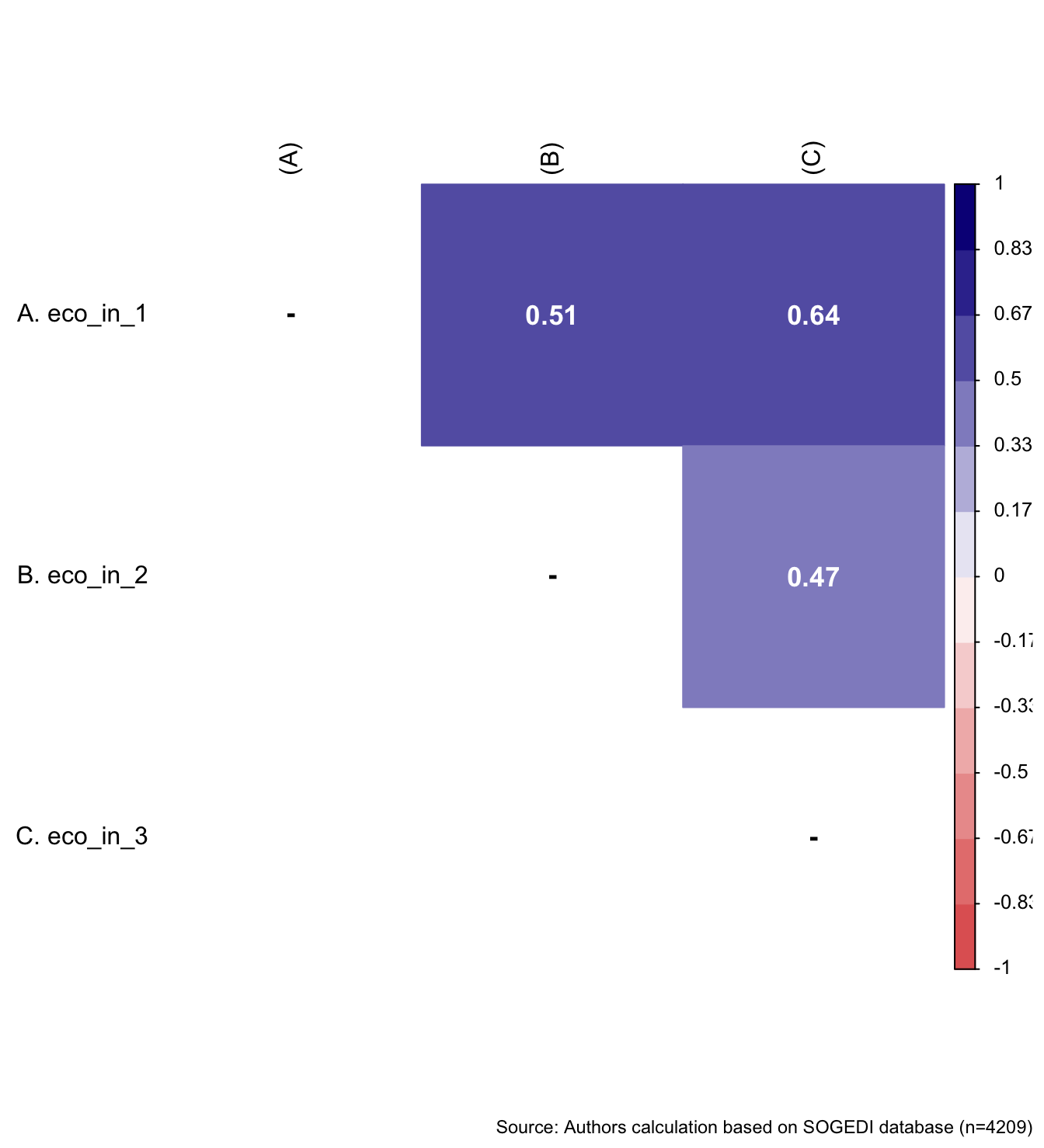
5.1.1 Perception of economic inequality in daily live
The items to capture individual subjective perception of daily economic inequality came from previous research from García-Castro et al. (2019). For the SOGEDI study we selected the items from the original scale that had the highest saturation on the construct and could potentially be more suitable for application in different countries.
Descriptive analysis
describe_kable(db_proc, c("eco_in_1", "eco_in_2", "eco_in_3"))| vars | n | mean | sd | median | trimmed | mad | min | max | range | skew | kurtosis | se | |
|---|---|---|---|---|---|---|---|---|---|---|---|---|---|
| eco_in_1 | 1 | 4209 | 5.789 | 1.410 | 6 | 6.007 | 1.483 | 1 | 7 | 6 | -1.167 | 0.961 | 0.022 |
| eco_in_2 | 2 | 4209 | 5.794 | 1.468 | 6 | 6.040 | 1.483 | 1 | 7 | 6 | -1.204 | 0.859 | 0.023 |
| eco_in_3 | 3 | 4209 | 5.734 | 1.557 | 6 | 6.009 | 1.483 | 1 | 7 | 6 | -1.251 | 0.954 | 0.024 |
wrap_elements(
    ~corrplot::corrplot(
      fit_correlations(db_proc, c("eco_in_1", "eco_in_2", "eco_in_3")),
      method = "color",
      type = "upper",
      col = colorRampPalette(c("#E16462", "white", "#0D0887"))(12),
      tl.pos = "lt",
      tl.col = "black",
      addrect = 2,
      rect.col = "black",
      addCoef.col = "white",
      cl.cex = 0.8,
      cl.align.text = 'l',
      number.cex = 1.1,
      na.label = "-",
      bg = "white"
    )
  ) + labs(caption = paste0(
    "Source: Authors calculation based on SOGEDI",
    " database (n=", nrow(db_proc), ")"
  ))
Reliability
mi_variable <- "eco_in"
result1 <- alphas(db_proc, c("eco_in_1", "eco_in_2", "eco_in_3"), mi_variable)

result1$raw_alpha
[1] 0.7778003result1$new_var_summary Min. 1st Qu. Median Mean 3rd Qu. Max.
1.000 5.000 6.000 5.773 7.000 7.000 Confirmatory Factor Analysis
Mardia’s test for evaluate multivariate normality.
mardia(db_proc[,c("eco_in_1", "eco_in_2", "eco_in_3")],
       na.rm = T, plot=T)
Call: mardia(x = db_proc[, c(“eco_in_1”, “eco_in_2”, “eco_in_3”)], na.rm = T, plot = T)
Mardia tests of multivariate skew and kurtosis Use describe(x) the to get univariate tests n.obs = 4209 num.vars = 3 b1p = 5.37 skew = 3767.2 with probability <= 0 small sample skew = 3771.23 with probability <= 0 b2p = 27.82 kurtosis = 75.95 with probability <= 0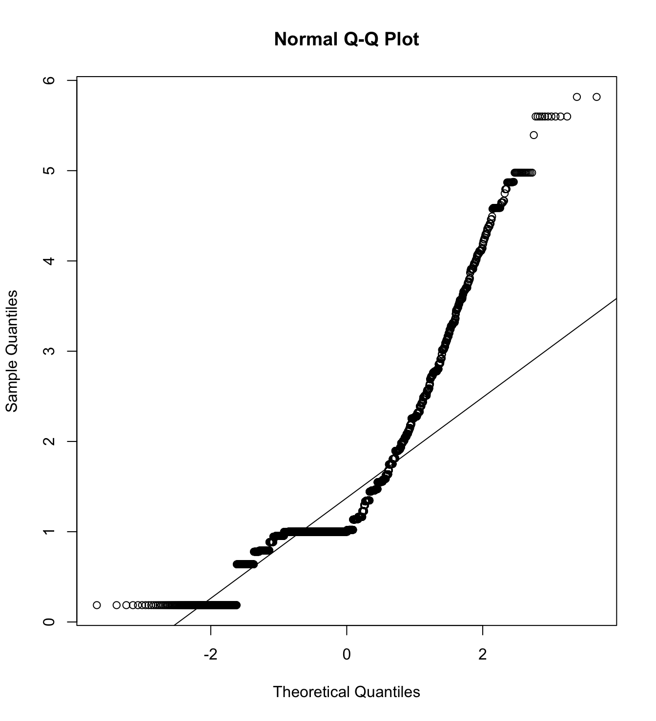
We first specify the factorial structure of the items, then fit models using a robust maximum likelihood estimator for the entire sample as well as for each country individually. The goodness of fit indicators are shown.
# model
model_cfa <- ' perc_eco_inequality =~ eco_in_1 + eco_in_2 + eco_in_3 '

# estimation
m1_cfa <- cfa(model = model_cfa,
              data = db_proc,
              estimator = "MLR",
              ordered = F,
              std.lv = F)

m1_cfa_arg <- cfa(model = model_cfa,
              data = subset(db_proc, country_residence_recoded == 1),
              estimator = "MLR",
              ordered = F,
              std.lv = F)

m1_cfa_cl <- cfa(model = model_cfa,
              data = subset(db_proc, country_residence_recoded == 3),
              estimator = "MLR",
              ordered = F,
              std.lv = F)

m1_cfa_col <- cfa(model = model_cfa,
              data = subset(db_proc, country_residence_recoded == 4),
              estimator = "MLR",
              ordered = F,
              std.lv = F)

m1_cfa_es <- cfa(model = model_cfa,
              data = subset(db_proc, country_residence_recoded == 9),
              estimator = "MLR",
              ordered = F,
              std.lv = F)

m1_cfa_mex <- cfa(model = model_cfa,
              data = subset(db_proc, country_residence_recoded == 13),
              estimator = "MLR",
              ordered = F,
std.lv = F) cfa_tab_fit(
models = list(m1_cfa, m1_cfa_arg, m1_cfa_cl, m1_cfa_col, m1_cfa_es, m1_cfa_mex),
country_names = c("Overall scores", "Argentina", "Chile", "Colombia", "Spain", "México")
)$fit_table| \(N\) | Estimator | \(\chi^2\) (df) | CFI | TLI | RMSEA 90% CI [Lower-Upper] | SRMR | AIC | |
|---|---|---|---|---|---|---|---|---|
| Overall scores | 4209 | ML | 0 (0) | 1 | 1 | 0 [0-0] | 0 | 42001.068 |
| Argentina | 807 | ML | 0 (0) | 1 | 1 | 0 [0-0] | 0 | 8145.822 |
| Chile | 883 | ML | 0 (0) | 1 | 1 | 0 [0-0] | 0 | 8857.224 |
| Colombia | 833 | ML | 0 (0) | 1 | 1 | 0 [0-0] | 0 | 8228.138 |
| Spain | 835 | ML | 0 (0) | 1 | 1 | 0 [0-0] | 0 | 8033.080 |
| México | 846 | ML | 0 (0) | 1 | 1 | 0 [0-0] | 0 | 8556.013 |
5.1.2 Socioeconomic inequality justification
The item to capture individual justification of socioeconomic inequality was created by the project team.
Descriptive analysis
5.1.3 Economic inequality collective action
The item to capture individual collective action toward economic inequality was adapted from Fresno-Díaz et al. (2023).
Descriptive analysis
5.1.4 Ambivalent classism
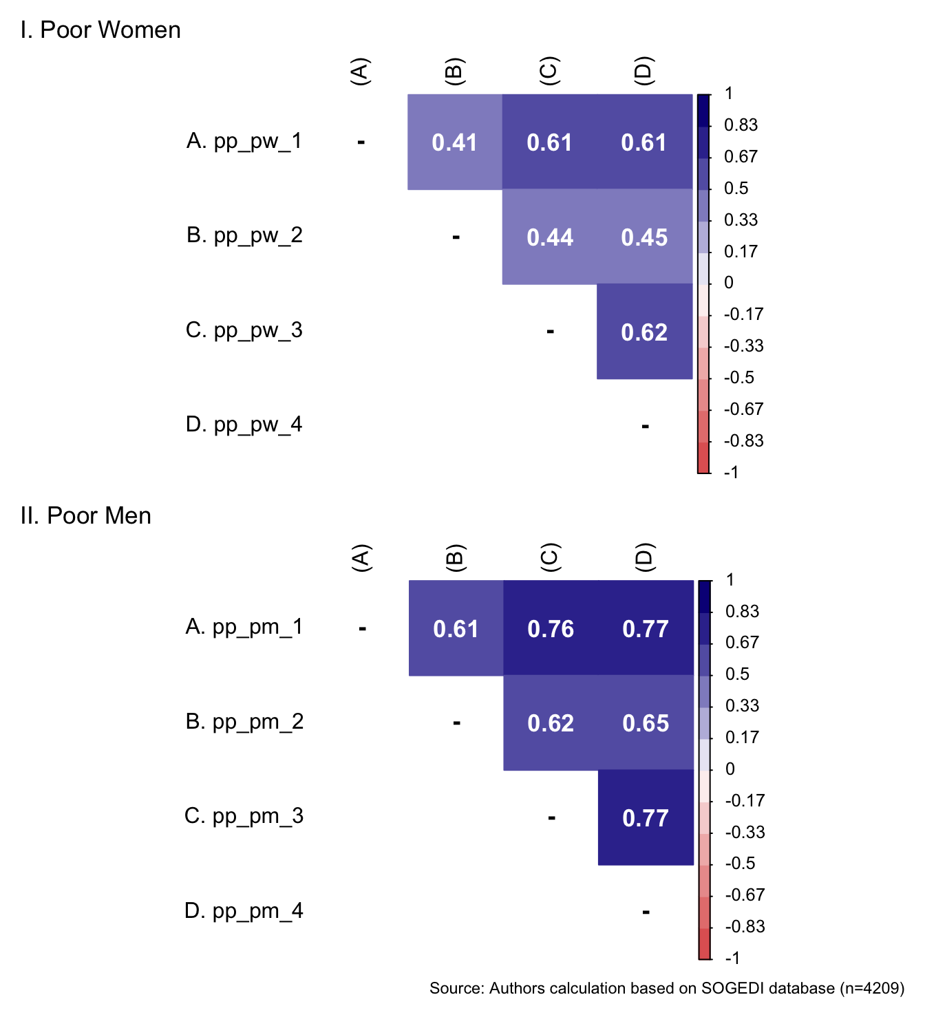
The items to capture ambivalent classism came from previous research from Sainz et al. (2021). For the SOGEDI study we used all items from the paternalistic/complementary dimensions of the scale adapted by the authors. For the hostile dimension, we selected the four items most strongly associated with the construct, based on the scale adaptation, while omitting items that could be misinterpreted in other spanish speaker contexts.
5.1.4.1 Protective paternalism toward poor women and men
Descriptive analysis
describe_kable(db_proc, c("pp_pw_1", "pp_pw_2", "pp_pw_3", "pp_pw_4", "pp_pm_1", "pp_pm_2", "pp_pm_3", "pp_pm_4"))| vars | n | mean | sd | median | trimmed | mad | min | max | range | skew | kurtosis | se | |
|---|---|---|---|---|---|---|---|---|---|---|---|---|---|
| pp_pw_1 | 1 | 4209 | 5.401 | 1.665 | 6 | 5.641 | 1.483 | 1 | 7 | 6 | -0.929 | 0.150 | 0.026 |
| pp_pw_2 | 2 | 4209 | 5.188 | 1.707 | 5 | 5.401 | 1.483 | 1 | 7 | 6 | -0.741 | -0.222 | 0.026 |
| pp_pw_3 | 3 | 4209 | 5.249 | 1.686 | 5 | 5.466 | 1.483 | 1 | 7 | 6 | -0.795 | -0.083 | 0.026 |
| pp_pw_4 | 4 | 4209 | 5.233 | 1.658 | 5 | 5.431 | 1.483 | 1 | 7 | 6 | -0.736 | -0.149 | 0.026 |
| pp_pm_1 | 5 | 4209 | 5.338 | 1.661 | 6 | 5.560 | 1.483 | 1 | 7 | 6 | -0.839 | -0.034 | 0.026 |
| pp_pm_2 | 6 | 4209 | 5.098 | 1.708 | 5 | 5.292 | 1.483 | 1 | 7 | 6 | -0.664 | -0.326 | 0.026 |
| pp_pm_3 | 7 | 4209 | 5.185 | 1.711 | 5 | 5.395 | 1.483 | 1 | 7 | 6 | -0.722 | -0.286 | 0.026 |
| pp_pm_4 | 8 | 4209 | 5.156 | 1.699 | 5 | 5.356 | 1.483 | 1 | 7 | 6 | -0.695 | -0.296 | 0.026 |
p1 <- wrap_elements(
  ~corrplot::corrplot(
    fit_correlations(db_proc, c("pp_pw_1", "pp_pw_2", "pp_pw_3", "pp_pw_4")),
    method = "color",
    type = "upper",
    col = colorRampPalette(c("#E16462", "white", "#0D0887"))(12),
    tl.pos = "lt",
    tl.col = "black",
    addrect = 2,
    rect.col = "black",
    addCoef.col = "white",
    cl.cex = 0.8,
    cl.align.text = 'l',
    number.cex = 1.1,
    na.label = "-",
    bg = "white"
  )
) + labs(title = 'I. Poor Women')

p2 <- wrap_elements(
  ~corrplot::corrplot(
    fit_correlations(db_proc, c("pp_pm_1", "pp_pm_2", "pp_pm_3", "pp_pm_4")),
    method = "color",
    type = "upper",
    col = colorRampPalette(c("#E16462", "white", "#0D0887"))(12),
    tl.pos = "lt",
    tl.col = "black",
    addrect = 2,
    rect.col = "black",
    addCoef.col = "white",
    cl.cex = 0.8,
    cl.align.text = 'l',
    number.cex = 1.1,
    na.label = "-",
    bg = "white"
  )
) + labs(title = 'II. Poor Men')

p1 / p2 + labs(
         caption = paste0(
  "Source: Authors calculation based on SOGEDI",
  " database (n=", nrow(db_proc), ")"
))
Reliability
mi_variable <- "pp_pw"
result2 <- alphas(db_proc, c("pp_pw_1", "pp_pw_2", "pp_pw_3", "pp_pw_4"), mi_variable)

result2$raw_alpha
[1] 0.8144432result2$new_var_summary Min. 1st Qu. Median Mean 3rd Qu. Max.
1.000 4.500 5.500 5.268 6.250 7.000 mi_variable <- "pp_pm"
result3 <- alphas(db_proc, c("pp_pm_1", "pp_pm_2", "pp_pm_3", "pp_pm_4"), mi_variable)
result3$raw_alpha[1] 0.901213result3$new_var_summary Min. 1st Qu. Median Mean 3rd Qu. Max.
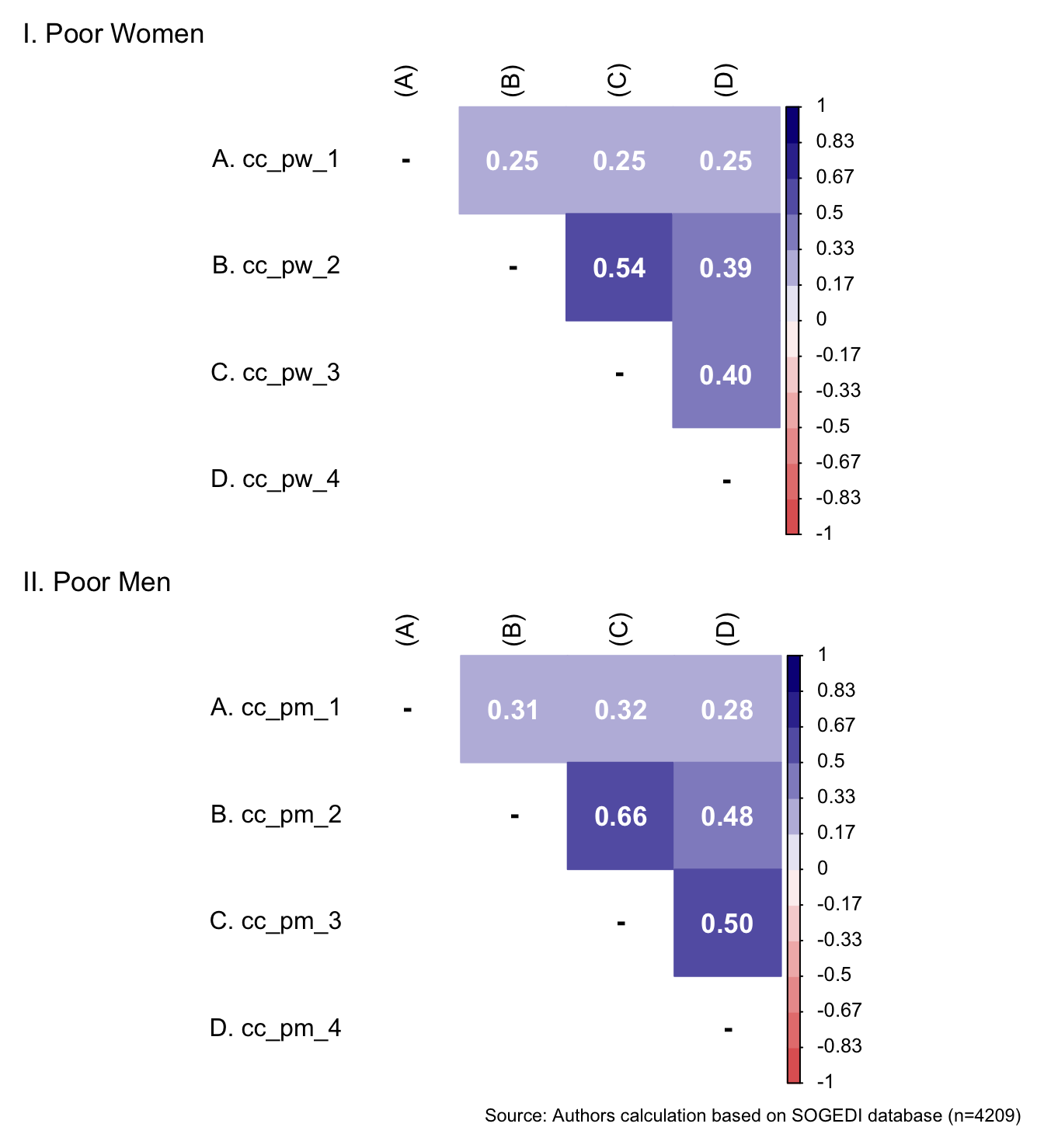
1.000 4.250 5.250 5.194 6.500 7.000 5.1.4.2 Complementary class diferenciation toward poor women and men
Descriptive analysis
describe_kable(db_proc, c("cc_pw_1", "cc_pw_2", "cc_pw_3", "cc_pw_4", "cc_pm_1", "cc_pm_2", "cc_pm_3", "cc_pm_4"))| vars | n | mean | sd | median | trimmed | mad | min | max | range | skew | kurtosis | se | |
|---|---|---|---|---|---|---|---|---|---|---|---|---|---|
| cc_pw_1 | 1 | 4209 | 5.353 | 1.585 | 6 | 5.536 | 1.483 | 1 | 7 | 6 | -0.711 | -0.236 | 0.024 |
| cc_pw_2 | 2 | 4209 | 3.702 | 1.680 | 4 | 3.658 | 1.483 | 1 | 7 | 6 | 0.055 | -0.498 | 0.026 |
| cc_pw_3 | 3 | 4209 | 3.858 | 1.808 | 4 | 3.822 | 1.483 | 1 | 7 | 6 | 0.020 | -0.792 | 0.028 |
| cc_pw_4 | 4 | 4209 | 4.340 | 1.869 | 4 | 4.425 | 1.483 | 1 | 7 | 6 | -0.307 | -0.828 | 0.029 |
| cc_pm_1 | 5 | 4209 | 4.874 | 1.676 | 5 | 4.993 | 1.483 | 1 | 7 | 6 | -0.333 | -0.702 | 0.026 |
| cc_pm_2 | 6 | 4209 | 3.524 | 1.609 | 4 | 3.462 | 1.483 | 1 | 7 | 6 | 0.125 | -0.411 | 0.025 |
| cc_pm_3 | 7 | 4209 | 3.593 | 1.680 | 4 | 3.530 | 1.483 | 1 | 7 | 6 | 0.150 | -0.560 | 0.026 |
| cc_pm_4 | 8 | 4209 | 4.137 | 1.820 | 4 | 4.172 | 1.483 | 1 | 7 | 6 | -0.136 | -0.827 | 0.028 |
p1 <- wrap_elements(
  ~corrplot::corrplot(
    fit_correlations(db_proc, c("cc_pw_1", "cc_pw_2", "cc_pw_3", "cc_pw_4")),
    method = "color",
    type = "upper",
    col = colorRampPalette(c("#E16462", "white", "#0D0887"))(12),
    tl.pos = "lt",
    tl.col = "black",
    addrect = 2,
    rect.col = "black",
    addCoef.col = "white",
    cl.cex = 0.8,
    cl.align.text = 'l',
    number.cex = 1.1,
    na.label = "-",
    bg = "white"
  )
) + labs(title = 'I. Poor Women')

p2 <- wrap_elements(
  ~corrplot::corrplot(
    fit_correlations(db_proc, c("cc_pm_1", "cc_pm_2", "cc_pm_3", "cc_pm_4")),
    method = "color",
    type = "upper",
    col = colorRampPalette(c("#E16462", "white", "#0D0887"))(12),
    tl.pos = "lt",
    tl.col = "black",
    addrect = 2,
    rect.col = "black",
    addCoef.col = "white",
    cl.cex = 0.8,
    cl.align.text = 'l',
    number.cex = 1.1,
    na.label = "-",
    bg = "white"
  )
) + labs(title = 'II. Poor Men')

p1 / p2 + labs(
         caption = paste0(
  "Source: Authors calculation based on SOGEDI",
  " database (n=", nrow(db_proc), ")"
))
Reliability
mi_variable <- "cc_pw"
result2 <- alphas(db_proc, c("cc_pw_1", "cc_pw_2", "cc_pw_3", "cc_pw_4"), mi_variable)

result2$raw_alpha
[1] 0.6841424result2$new_var_summary Min. 1st Qu. Median Mean 3rd Qu. Max.
1.000 3.500 4.250 4.313 5.000 7.000 mi_variable <- "cc_pm"
result3 <- alphas(db_proc, c("cc_pm_1", "cc_pm_2", "cc_pm_3", "cc_pm_4"), mi_variable)
result3$raw_alpha[1] 0.7443716result3$new_var_summary Min. 1st Qu. Median Mean 3rd Qu. Max.
1.000 3.250 4.000 4.032 4.750 7.000 5.1.4.3 Hostile classism toward poor women and men
Descriptive analysis
describe_kable(db_proc, c("hc_pw_1","hc_pw_2","hc_pw_3","hc_pw_4", "hc_pm_1","hc_pm_2","hc_pm_3","hc_pm_4"))| vars | n | mean | sd | median | trimmed | mad | min | max | range | skew | kurtosis | se | |
|---|---|---|---|---|---|---|---|---|---|---|---|---|---|
| hc_pw_1 | 1 | 4209 | 2.474 | 1.600 | 2 | 2.256 | 1.483 | 1 | 7 | 6 | 0.871 | -0.105 | 0.025 |
| hc_pw_2 | 2 | 4209 | 2.929 | 1.862 | 3 | 2.714 | 2.965 | 1 | 7 | 6 | 0.610 | -0.734 | 0.029 |
| hc_pw_3 | 3 | 4209 | 2.616 | 1.697 | 2 | 2.400 | 1.483 | 1 | 7 | 6 | 0.771 | -0.367 | 0.026 |
| hc_pw_4 | 4 | 4209 | 3.189 | 1.817 | 3 | 3.039 | 2.965 | 1 | 7 | 6 | 0.372 | -0.845 | 0.028 |
| hc_pm_1 | 5 | 4209 | 3.064 | 1.731 | 3 | 2.917 | 1.483 | 1 | 7 | 6 | 0.408 | -0.717 | 0.027 |
| hc_pm_2 | 6 | 4209 | 3.229 | 1.804 | 3 | 3.084 | 1.483 | 1 | 7 | 6 | 0.373 | -0.805 | 0.028 |
| hc_pm_3 | 7 | 4209 | 3.118 | 1.730 | 3 | 2.978 | 1.483 | 1 | 7 | 6 | 0.373 | -0.728 | 0.027 |
| hc_pm_4 | 8 | 4209 | 3.618 | 1.831 | 4 | 3.547 | 1.483 | 1 | 7 | 6 | 0.116 | -0.919 | 0.028 |
p1 <- wrap_elements(
  ~corrplot::corrplot(
    fit_correlations(db_proc, c("hc_pw_1", "h_pw_2", "hc_pw_3", "hc_pw_4")),
    method = "color",
    type = "upper",
    col = colorRampPalette(c("#E16462", "white", "#0D0887"))(12),
    tl.pos = "lt",
    tl.col = "black",
    addrect = 2,
    rect.col = "black",
    addCoef.col = "white",
    cl.cex = 0.8,
    cl.align.text = 'l',
    number.cex = 1.1,
    na.label = "-",
    bg = "white"
  )
) + labs(title = 'I. Poor Women')

p2 <- wrap_elements(
  ~corrplot::corrplot(
    fit_correlations(db_proc, c("hc_pm_1", "hc_pm_2", "hc_pm_3", "hc_pm_4")),
    method = "color",
    type = "upper",
    col = colorRampPalette(c("#E16462", "white", "#0D0887"))(12),
    tl.pos = "lt",
    tl.col = "black",
    addrect = 2,
    rect.col = "black",
    addCoef.col = "white",
    cl.cex = 0.8,
    cl.align.text = 'l',
    number.cex = 1.1,
    na.label = "-",
    bg = "white"
  )
) + labs(title = 'II. Poor Men')

p1 / p2 + labs(
         caption = paste0(
  "Source: Authors calculation based on SOGEDI",
  " database (n=", nrow(db_proc), ")"
))
Reliability
mi_variable <- "hc_pw"
result2 <- alphas(db_proc, c("hc_pw_1","hc_pw_2","hc_pw_3","hc_pw_4"), mi_variable)

result2$raw_alpha
[1] 0.7858148result2$new_var_summary Min. 1st Qu. Median Mean 3rd Qu. Max.
1.000 1.750 2.750 2.802 3.750 7.000 mi_variable <- "hc_pm"
result3 <- alphas(db_proc, c("hc_pm_1","hc_pm_2","hc_pm_3","hc_pm_4"), mi_variable)
result3$raw_alpha[1] 0.8526135result3$new_var_summary Min. 1st Qu. Median Mean 3rd Qu. Max.
1.000 2.000 3.250 3.257 4.250 7.000 Confirmatory Factor Analysis
Ambilavent classim with woman as target
Mardia’s test for evaluate multivariate normality.
mardia(db_proc[,c("pp_pw_1", "pp_pw_2", "pp_pw_3", "pp_pw_4",
                  "cc_pw_1", "cc_pw_2", "cc_pw_3", "cc_pw_4",
                  "hc_pw_1", "hc_pw_2", "hc_pw_3", "hc_pw_4")],
       na.rm = T, plot=T)
Call: mardia(x = db_proc[, c(“pp_pw_1”, “pp_pw_2”, “pp_pw_3”, “pp_pw_4”, “cc_pw_1”, “cc_pw_2”, “cc_pw_3”, “cc_pw_4”, “hc_pw_1”, “hc_pw_2”, “hc_pw_3”, “hc_pw_4”)], na.rm = T, plot = T)
Mardia tests of multivariate skew and kurtosis Use describe(x) the to get univariate tests n.obs = 4209 num.vars = 12 b1p = 9.08 skew = 6371.73 with probability <= 0 small sample skew = 6376.97 with probability <= 0 b2p = 210.51 kurtosis = 75.24 with probability <= 0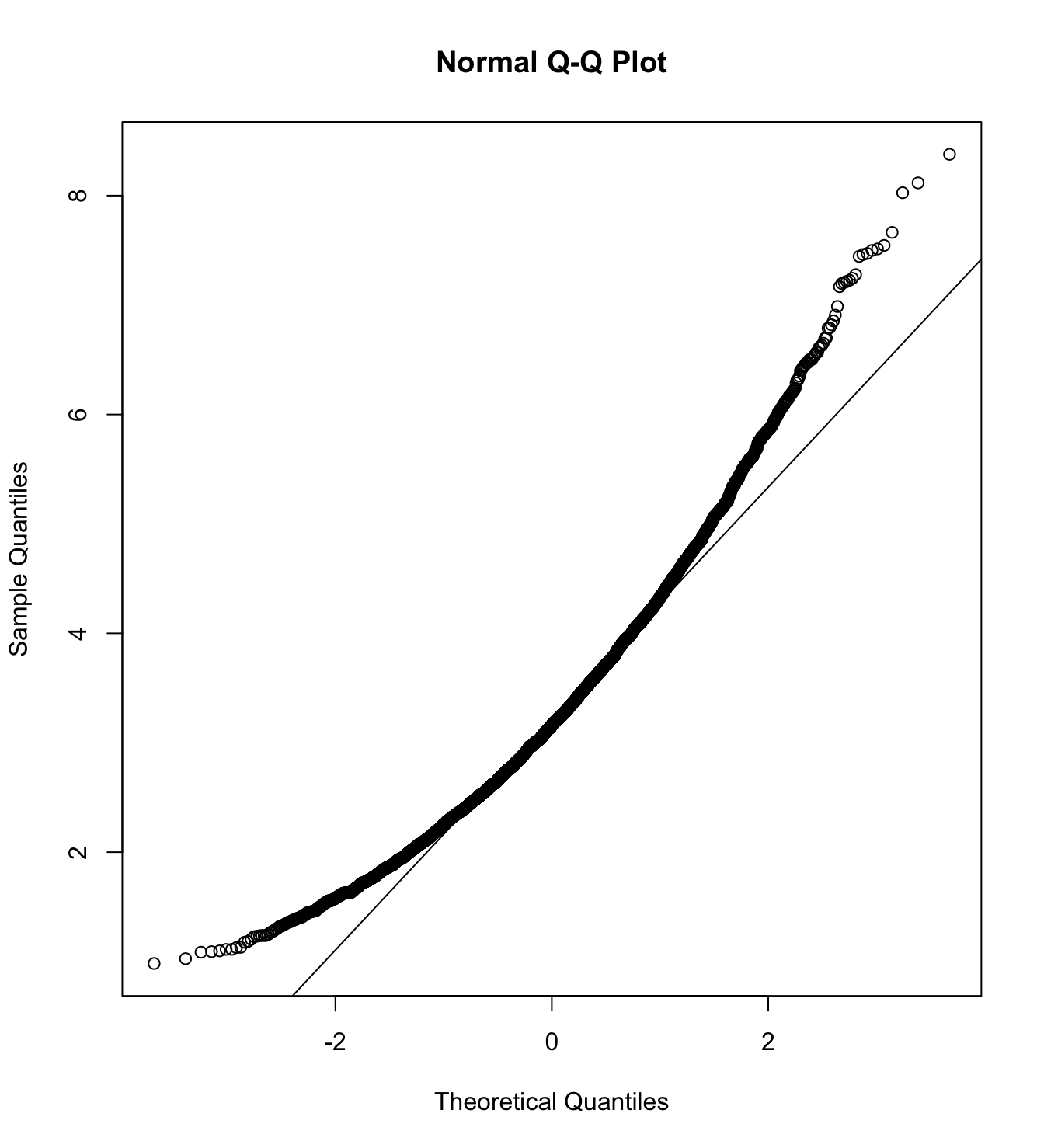
We first specify the factorial structure of the items, then fit models using a robust maximum likelihood estimator for the entire sample as well as for each country individually. The goodness of fit indicators are shown.
# model
model_cfa <- '
  aci_pp =~ pp_pw_1 + pp_pw_2 + pp_pw_3 + pp_pw_4
  aci_cc =~ cc_pw_1 + cc_pw_2 + cc_pw_3 + cc_pw_4
  aci_hc =~ hc_pw_1 + hc_pw_2 + hc_pw_3 + hc_pw_4
  aci =~ aci_pp + aci_cc + aci_hc '

# estimation
m2_cfa <- cfa(model = model_cfa,
              data = db_proc,
              estimator = "MLR",
              ordered = F,
              std.lv = F)

m2_cfa_arg <- cfa(model = model_cfa,
              data = subset(db_proc, country_residence_recoded == 1),
              estimator = "MLR",
              ordered = F,
              std.lv = F)

m2_cfa_cl <- cfa(model = model_cfa,
              data = subset(db_proc, country_residence_recoded == 3),
              estimator = "MLR",
              ordered = F,
              std.lv = F)

m2_cfa_col <- cfa(model = model_cfa,
              data = subset(db_proc, country_residence_recoded == 4),
              estimator = "MLR",
              ordered = F,
              std.lv = F)

m2_cfa_es <- cfa(model = model_cfa,
              data = subset(db_proc, country_residence_recoded == 9),
              estimator = "MLR",
              ordered = F,
              std.lv = F)

m2_cfa_mex <- cfa(model = model_cfa,
              data = subset(db_proc, country_residence_recoded == 13),
              estimator = "MLR",
              ordered = F,
              std.lv = F)
Ambilavent classim with men as target
Mardia’s test for evaluate multivariate normality.
mardia(db_proc[,c("pp_pm_1", "pp_pm_2", "pp_pm_3", "pp_pm_4",
                  "cc_pm_1", "cc_pm_2", "cc_pm_3", "cc_pm_4",
                  "hc_pm_1", "hc_pm_2", "hc_pm_3", "hc_pm_4")],
       na.rm = T, plot=T)
Call: mardia(x = db_proc[, c(“pp_pm_1”, “pp_pm_2”, “pp_pm_3”, “pp_pm_4”, “cc_pm_1”, “cc_pm_2”, “cc_pm_3”, “cc_pm_4”, “hc_pm_1”, “hc_pm_2”, “hc_pm_3”, “hc_pm_4”)], na.rm = T, plot = T)
Mardia tests of multivariate skew and kurtosis Use describe(x) the to get univariate tests n.obs = 4209 num.vars = 12 b1p = 8.22 skew = 5768.28 with probability <= 0 small sample skew = 5773.03 with probability <= 0 b2p = 234.53 kurtosis = 117.74 with probability <= 0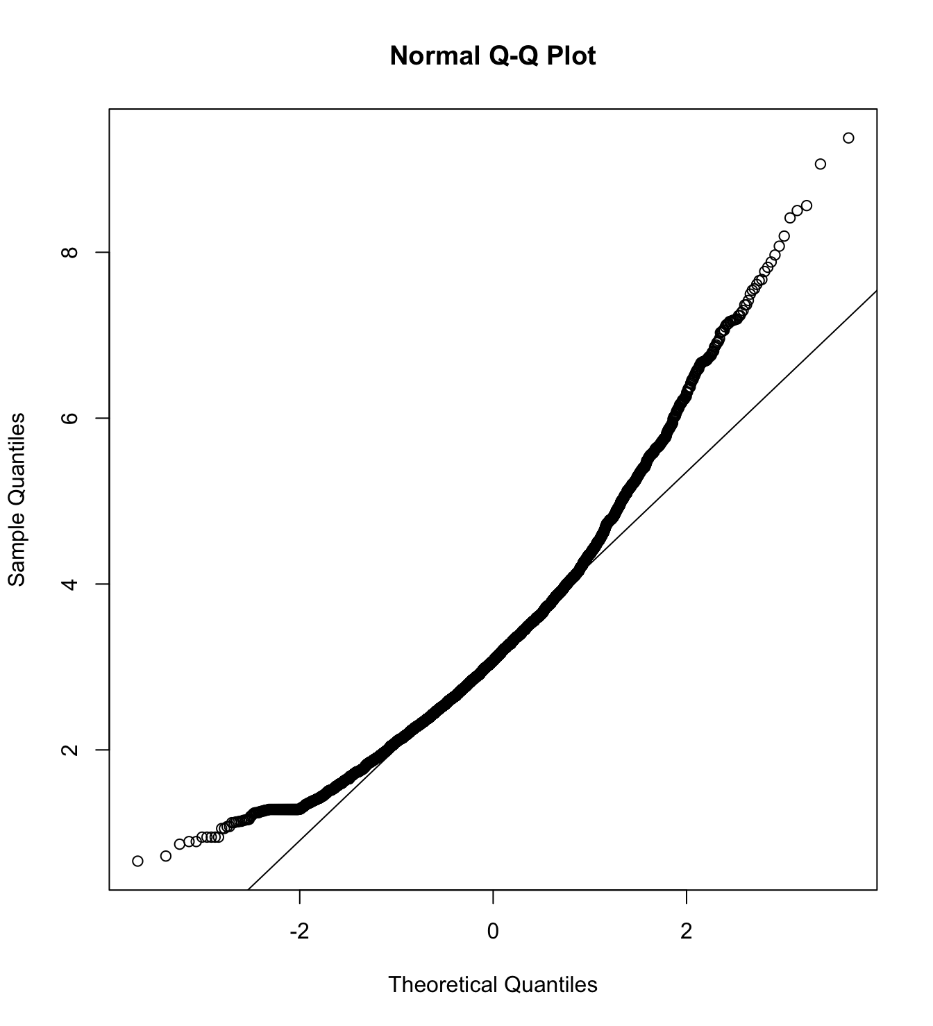
We first specify the factorial structure of the items, then fit models using a robust maximum likelihood estimator for the entire sample as well as for each country individually. The goodness of fit indicators are shown.
# model
model_cfa <- '
  aci_pp =~ pp_pm_1 + pp_pm_2 + pp_pm_3 + pp_pm_4
  aci_cc =~ cc_pm_1 + cc_pm_2 + cc_pm_3 + cc_pm_4
  aci_hc =~ hc_pm_1 + hc_pm_2 + hc_pm_3 + hc_pm_4
  aci =~ aci_pp + aci_cc + aci_hc '

# estimation
m3_cfa <- cfa(model = model_cfa,
              data = db_proc,
              estimator = "MLR",
              ordered = F,
              std.lv = F)

m3_cfa_arg <- cfa(model = model_cfa,
              data = subset(db_proc, country_residence_recoded == 1),
              estimator = "MLR",
              ordered = F,
              std.lv = F)

m3_cfa_cl <- cfa(model = model_cfa,
              data = subset(db_proc, country_residence_recoded == 3),
              estimator = "MLR",
              ordered = F,
              std.lv = F)

m3_cfa_col <- cfa(model = model_cfa,
              data = subset(db_proc, country_residence_recoded == 4),
              estimator = "MLR",
              ordered = F,
              std.lv = F)

m3_cfa_es <- cfa(model = model_cfa,
              data = subset(db_proc, country_residence_recoded == 9),
              estimator = "MLR",
              ordered = F,
              std.lv = F)

m3_cfa_mex <- cfa(model = model_cfa,
              data = subset(db_proc, country_residence_recoded == 13),
              estimator = "MLR",
              ordered = F,
              std.lv = F)
colnames_fit <- c("","Target","$N$","Estimator","$\\chi^2$ (df)","CFI","TLI","RMSEA 90% CI [Lower-Upper]", "SRMR", "AIC")
bind_rows(
cfa_tab_fit(
models = list(m2_cfa, m2_cfa_arg, m2_cfa_cl, m2_cfa_col, m2_cfa_es, m2_cfa_mex),
country_names = c("Overall scores", "Argentina", "Chile", "Colombia", "Spain", "México")
)$sum_fit %>%
mutate(target = "Poor Women")
,
cfa_tab_fit(
models = list(m3_cfa, m3_cfa_arg, m3_cfa_cl, m3_cfa_col, m3_cfa_es, m3_cfa_mex),
country_names = c("Overall scores", "Argentina", "Chile", "Colombia", "Spain", "México")
)$sum_fit %>%
mutate(target = "Poor Men")
) %>%
select(country, target, everything()) %>%
mutate(country = factor(country, levels = c("Overall scores", "Argentina", "Chile", "Colombia", "Spain", "México"))) %>%
group_by(country) %>%
arrange(country) %>%
mutate(country = if_else(duplicated(country), NA, country)) %>%
kableExtra::kable(
format = "markdown",
digits = 3,
booktabs = TRUE,
col.names = colnames_fit,
caption = NULL
) %>%
kableExtra::kable_styling(
full_width = TRUE,
font_size = 11,
latex_options = "HOLD_position",
bootstrap_options = c("striped", "bordered")
) %>%
kableExtra::collapse_rows(columns = 1)| Target | \(N\) | Estimator | \(\chi^2\) (df) | CFI | TLI | RMSEA 90% CI [Lower-Upper] | SRMR | AIC | |
|---|---|---|---|---|---|---|---|---|---|
| Overall scores | Poor Women | 4209 | ML | 963.662 (51) *** | 0.938 | 0.919 | 0.065 [0.062-0.069] | 0.061 | 184251.80 |
| Poor Men | 4209 | ML | 875.132 (51) *** | 0.965 | 0.955 | 0.062 [0.058-0.066] | 0.061 | 175230.23 | |
| Argentina | Poor Women | 807 | ML | 265.228 (51) *** | 0.924 | 0.901 | 0.072 [0.064-0.081] | 0.072 | 35713.32 |
| Poor Men | 807 | ML | 295.154 (51) *** | 0.945 | 0.929 | 0.077 [0.069-0.086] | 0.073 | 34033.94 | |
| Chile | Poor Women | 883 | ML | 331.766 (51) *** | 0.911 | 0.885 | 0.079 [0.071-0.087] | 0.076 | 38590.58 |
| Poor Men | 883 | ML | 202.945 (51) *** | 0.968 | 0.959 | 0.058 [0.05-0.067] | 0.060 | 36691.01 | |
| Colombia | Poor Women | 833 | ML | 229.327 (51) *** | 0.932 | 0.911 | 0.065 [0.056-0.073] | 0.063 | 36271.89 |
| Poor Men | 833 | ML | 208.431 (51) *** | 0.962 | 0.951 | 0.061 [0.052-0.07] | 0.061 | 34976.60 | |
| Spain | Poor Women | 835 | ML | 178.617 (51) *** | 0.963 | 0.952 | 0.055 [0.046-0.064] | 0.057 | 33998.19 |
| Poor Men | 835 | ML | 241.732 (51) *** | 0.967 | 0.957 | 0.067 [0.059-0.076] | 0.061 | 32088.39 | |
| México | Poor Women | 846 | ML | 203.834 (51) *** | 0.934 | 0.915 | 0.06 [0.051-0.068] | 0.059 | 38260.01 |
| Poor Men | 846 | ML | 237.3 (51) *** | 0.957 | 0.945 | 0.066 [0.057-0.074] | 0.064 | 36206.58 |
5.2 Block 2. Gender inequality / Attitudes
5.2.1 Ambivalent sexism
The items to capture ambivalent sexism came from previous research from Rollero et al. (2014) and Rodríguez-Castro et al. (2009).
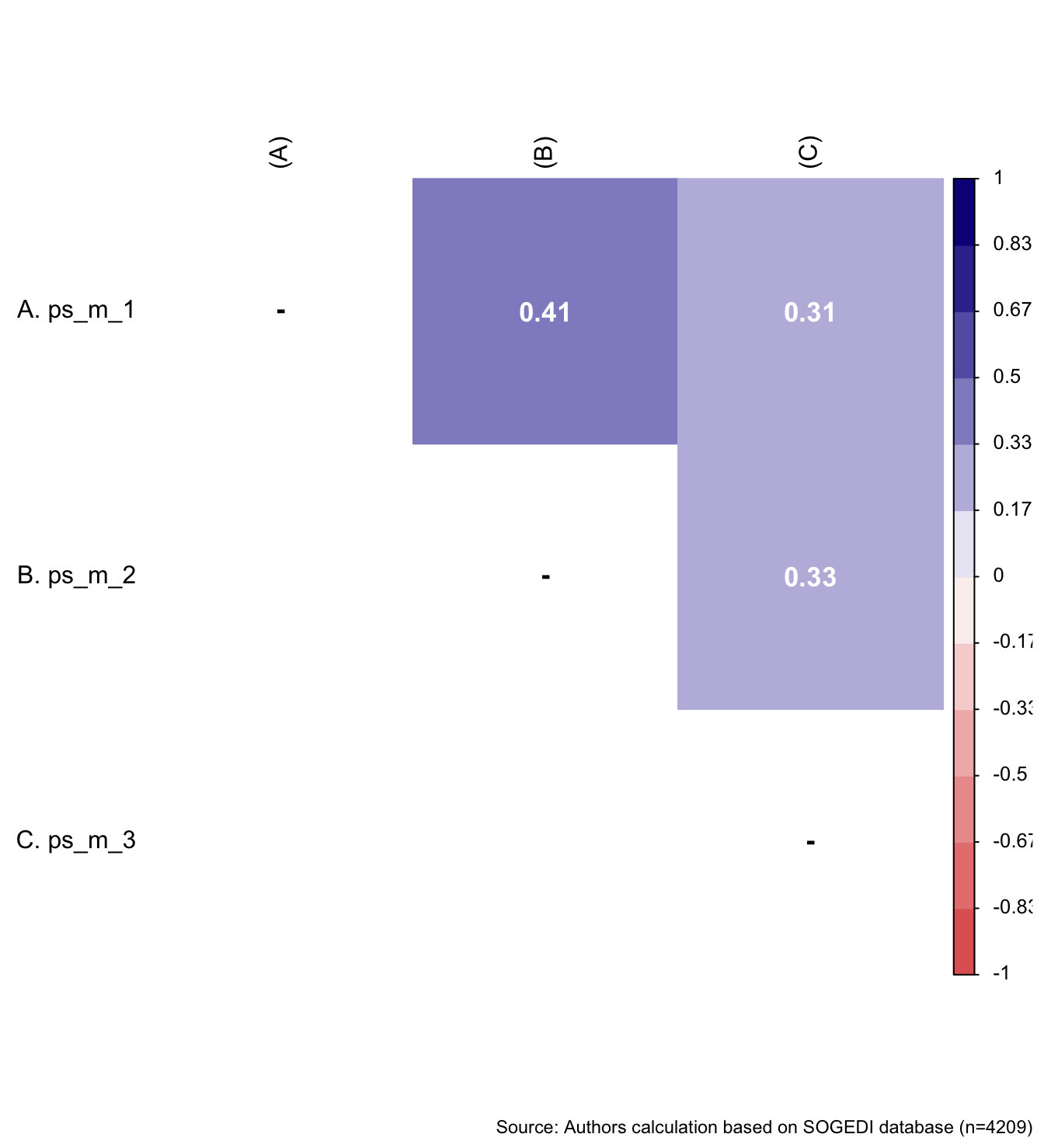
5.2.1.1 Paternalism sexism toward women
Descriptive results
describe_kable(db_proc, c("ps_m_1", "ps_m_2", "ps_m_3"))| vars | n | mean | sd | median | trimmed | mad | min | max | range | skew | kurtosis | se | |
|---|---|---|---|---|---|---|---|---|---|---|---|---|---|
| ps_m_1 | 1 | 4209 | 4.926 | 1.983 | 5 | 5.157 | 2.965 | 1 | 7 | 6 | -0.598 | -0.763 | 0.031 |
| ps_m_2 | 2 | 4209 | 3.480 | 2.280 | 4 | 3.351 | 4.448 | 1 | 7 | 6 | 0.284 | -1.399 | 0.035 |
| ps_m_3 | 3 | 4209 | 3.429 | 1.881 | 4 | 3.310 | 1.483 | 1 | 7 | 6 | 0.225 | -0.937 | 0.029 |
wrap_elements(
    ~corrplot::corrplot(
      fit_correlations(db_proc, c("ps_m_1", "ps_m_2", "ps_m_3")),
      method = "color",
      type = "upper",
      col = colorRampPalette(c("#E16462", "white", "#0D0887"))(12),
      tl.pos = "lt",
      tl.col = "black",
      addrect = 2,
      rect.col = "black",
      addCoef.col = "white",
      cl.cex = 0.8,
      cl.align.text = 'l',
      number.cex = 1.1,
      na.label = "-",
      bg = "white"
    )
  ) + labs(caption = paste0(
    "Source: Authors calculation based on SOGEDI",
    " database (n=", nrow(db_proc), ")"
  ))
Reliability
mi_variable <- "ps_m"
result2 <- alphas(db_proc, c("ps_m_1", "ps_m_2", "ps_m_3"), mi_variable)

result2$raw_alpha
[1] 0.6148687result2$new_var_summary Min. 1st Qu. Median Mean 3rd Qu. Max.
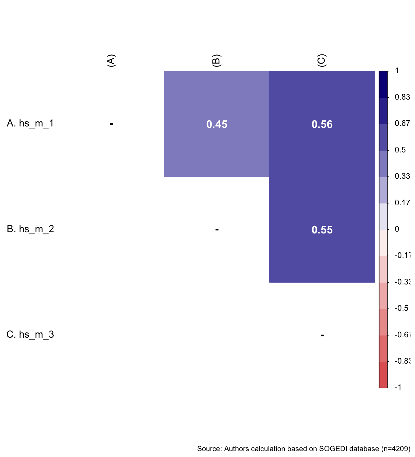
1.000 3.000 4.000 3.945 5.000 7.000 5.2.1.2 Hostility sexism toward women
Descriptive results
describe_kable(db_proc, c("hs_m_1", "hs_m_2", "hs_m_3"))| vars | n | mean | sd | median | trimmed | mad | min | max | range | skew | kurtosis | se | |
|---|---|---|---|---|---|---|---|---|---|---|---|---|---|
| hs_m_1 | 1 | 4209 | 3.370 | 1.818 | 4 | 3.260 | 1.483 | 1 | 7 | 6 | 0.234 | -0.926 | 0.028 |
| hs_m_2 | 2 | 4209 | 2.914 | 1.776 | 3 | 2.725 | 2.965 | 1 | 7 | 6 | 0.571 | -0.675 | 0.027 |
| hs_m_3 | 3 | 4209 | 3.267 | 1.958 | 3 | 3.109 | 2.965 | 1 | 7 | 6 | 0.349 | -1.054 | 0.030 |
wrap_elements(
    ~corrplot::corrplot(
      fit_correlations(db_proc, c("hs_m_1", "hs_m_2", "hs_m_3")),
      method = "color",
      type = "upper",
      col = colorRampPalette(c("#E16462", "white", "#0D0887"))(12),
      tl.pos = "lt",
      tl.col = "black",
      addrect = 2,
      rect.col = "black",
      addCoef.col = "white",
      cl.cex = 0.8,
      cl.align.text = 'l',
      number.cex = 1.1,
      na.label = "-",
      bg = "white"
    )
  ) + labs(caption = paste0(
    "Source: Authors calculation based on SOGEDI",
    " database (n=", nrow(db_proc), ")"
  ))
Reliability
mi_variable <- "hs_m"
result2 <- alphas(db_proc, c("hs_m_1", "hs_m_2", "hs_m_3"), mi_variable)

result2$raw_alpha
[1] 0.7658961result2$new_var_summary Min. 1st Qu. Median Mean 3rd Qu. Max.
1.000 2.000 3.000 3.184 4.333 7.000 Confirmatory Factor Analysis
Mardia’s test for evaluate multivariate normality.
mardia(db_proc[,c("ps_m_1", "ps_m_2", "ps_m_3",
                  "hs_m_1", "hs_m_2", "hs_m_3")],
       na.rm = T, plot=T)
Call: mardia(x = db_proc[, c(“ps_m_1”, “ps_m_2”, “ps_m_3”, “hs_m_1”, “hs_m_2”, “hs_m_3”)], na.rm = T, plot = T)
Mardia tests of multivariate skew and kurtosis Use describe(x) the to get univariate tests n.obs = 4209 num.vars = 6 b1p = 1.55 skew = 1087.81 with probability <= 0.000000000000000000000000000000000000000000000000000000000000000000000000000000000000000000000000000000000000000000000000000000000000000000000000000000000000000000000000000000000000000000000043 small sample skew = 1088.81 with probability <= 0.000000000000000000000000000000000000000000000000000000000000000000000000000000000000000000000000000000000000000000000000000000000000000000000000000000000000000000000000000000000000000000000027 b2p = 50.82 kurtosis = 9.35 with probability <= 0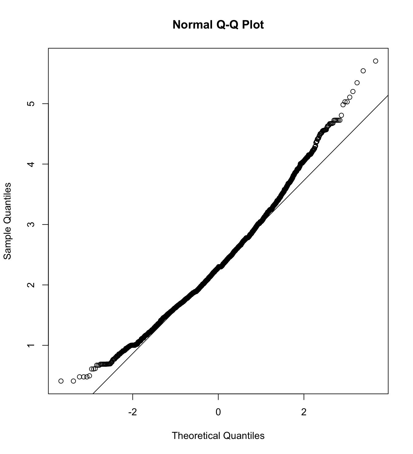
We first specify the factorial structure of the items, then fit models using a robust maximum likelihood estimator for the entire sample as well as for each country individually. The goodnes of fit indicators are shown.
# model
model_cfa <- '
  psm =~ ps_m_1 + ps_m_2 + ps_m_3
  hsm =~ hs_m_1 + hs_m_2 + hs_m_3
  asi =~ psm + hsm '

# estimation
m4_cfa <- cfa(model = model_cfa,
              data = db_proc,
              estimator = "MLR",
              ordered = F,
              std.lv = F)

m4_cfa_arg <- cfa(model = model_cfa,
              data = subset(db_proc, country_residence_recoded == 1),
              estimator = "MLR",
              ordered = F,
              std.lv = F)

m4_cfa_cl <- cfa(model = model_cfa,
              data = subset(db_proc, country_residence_recoded == 3),
              estimator = "MLR",
              ordered = F,
              std.lv = F)

m4_cfa_col <- cfa(model = model_cfa,
              data = subset(db_proc, country_residence_recoded == 4),
              estimator = "MLR",
              ordered = F,
              std.lv = F)

m4_cfa_es <- cfa(model = model_cfa,
              data = subset(db_proc, country_residence_recoded == 9),
              estimator = "MLR",
              ordered = F,
              std.lv = F)

m4_cfa_mex <- cfa(model = model_cfa,
              data = subset(db_proc, country_residence_recoded == 13),
              estimator = "MLR",
              ordered = F,
std.lv = F) cfa_tab_fit(
models = list(m4_cfa, m4_cfa_arg, m4_cfa_cl, m4_cfa_col, m4_cfa_es, m4_cfa_mex),
country_names = c("Overall scores", "Argentina", "Chile", "Colombia", "Spain", "México")
)$fit_table| \(N\) | Estimator | \(\chi^2\) (df) | CFI | TLI | RMSEA 90% CI [Lower-Upper] | SRMR | AIC | |
|---|---|---|---|---|---|---|---|---|
| Overall scores | 4209 | ML | 76.711 (7) *** | 0.987 | 0.972 | 0.049 [0.039-0.059] | 0.025 | 100051.14 |
| Argentina | 807 | ML | 6.668 (7) | 1.000 | 1.001 | 0 [0-0.042] | 0.015 | 19274.62 |
| Chile | 883 | ML | 34.958 (7) *** | 0.972 | 0.941 | 0.067 [0.046-0.09] | 0.032 | 21052.17 |
| Colombia | 833 | ML | 24.371 (7) *** | 0.979 | 0.955 | 0.055 [0.032-0.079] | 0.034 | 19686.31 |
| Spain | 835 | ML | 22.911 (7) ** | 0.988 | 0.974 | 0.052 [0.029-0.077] | 0.037 | 18591.20 |
| México | 846 | ML | 35.833 (7) *** | 0.964 | 0.923 | 0.07 [0.048-0.093] | 0.041 | 20419.26 |
5.2.2 Perception of gender inequality
We selected six items from the original scale developed by Schwartz-Salazar et al. (2024) that have several subdimensions. The reduced scale has not being published before so we will explore the factor structure of this four items.
Descriptive results
describe_kable(db_proc, c("gen_in_1", "gen_in_2", "gen_in_3", "gen_in_4", "gen_in_5", "gen_in_6"))| vars | n | mean | sd | median | trimmed | mad | min | max | range | skew | kurtosis | se | |
|---|---|---|---|---|---|---|---|---|---|---|---|---|---|
| gen_in_1 | 1 | 4209 | 5.345 | 1.792 | 6 | 5.631 | 1.483 | 1 | 7 | 6 | -0.995 | 0.060 | 0.028 |
| gen_in_2 | 2 | 4209 | 5.553 | 1.588 | 6 | 5.814 | 1.483 | 1 | 7 | 6 | -1.152 | 0.773 | 0.024 |
| gen_in_3 | 3 | 4209 | 4.694 | 1.939 | 5 | 4.868 | 1.483 | 1 | 7 | 6 | -0.521 | -0.801 | 0.030 |
| gen_in_4 | 4 | 4209 | 4.404 | 2.061 | 5 | 4.505 | 2.965 | 1 | 7 | 6 | -0.358 | -1.093 | 0.032 |
| gen_in_5 | 5 | 4209 | 3.941 | 2.033 | 4 | 3.927 | 2.965 | 1 | 7 | 6 | -0.046 | -1.160 | 0.031 |
| gen_in_6 | 6 | 4209 | 4.440 | 1.931 | 5 | 4.549 | 1.483 | 1 | 7 | 6 | -0.400 | -0.877 | 0.030 |
wrap_elements(
    ~corrplot::corrplot(
      fit_correlations(db_proc, c("gen_in_1", "gen_in_2", "gen_in_3", "gen_in_4", "gen_in_5", "gen_in_6")),
      method = "color",
      type = "upper",
      col = colorRampPalette(c("#E16462", "white", "#0D0887"))(12),
      tl.pos = "lt",
      tl.col = "black",
      addrect = 2,
      rect.col = "black",
      addCoef.col = "white",
      cl.cex = 0.8,
      cl.align.text = 'l',
      number.cex = 1.1,
      na.label = "-",
      bg = "white"
    )
  ) + labs(caption = paste0(
    "Source: Authors calculation based on SOGEDI",
    " database (n=", nrow(db_proc), ")"
  ))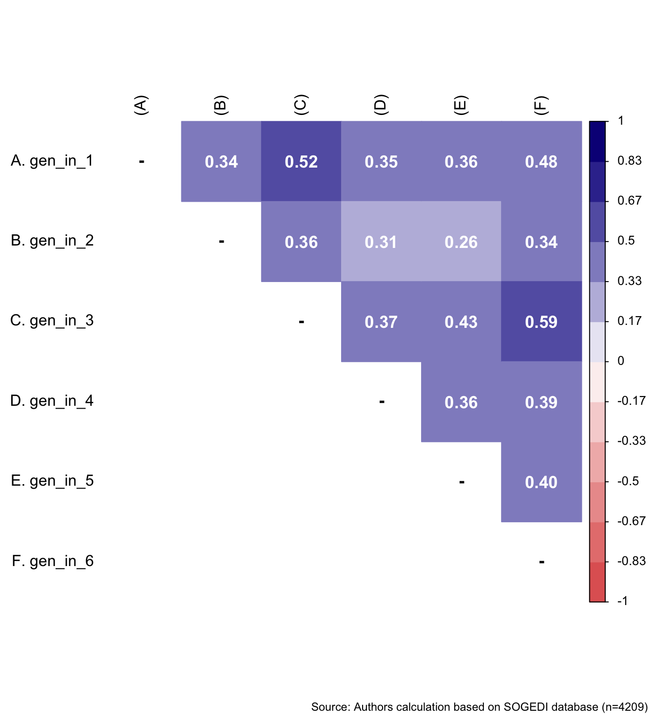
Reliability
mi_variable <- "gen_in"
result2 <- alphas(db_proc, c("gen_in_1", "gen_in_2", "gen_in_3", "gen_in_4", "gen_in_5", "gen_in_6"), mi_variable)

result2$raw_alpha
[1] 0.7923002result2$new_var_summary Min. 1st Qu. Median Mean 3rd Qu. Max.
1.000 3.833 4.833 4.730 5.667 7.000 Confirmatory factor analysis
Mardia’s test for evaluate multivariate normality.
mardia(db_proc[,c("gen_in_1", "gen_in_2", "gen_in_3",
                  "gen_in_4", "gen_in_5", "gen_in_6")],
       na.rm = T, plot=T)
Call: mardia(x = db_proc[, c(“gen_in_1”, “gen_in_2”, “gen_in_3”, “gen_in_4”, “gen_in_5”, “gen_in_6”)], na.rm = T, plot = T)
Mardia tests of multivariate skew and kurtosis Use describe(x) the to get univariate tests n.obs = 4209 num.vars = 6 b1p = 3.68 skew = 2584.66 with probability <= 0 small sample skew = 2587.03 with probability <= 0 b2p = 58.55 kurtosis = 34.94 with probability <= 0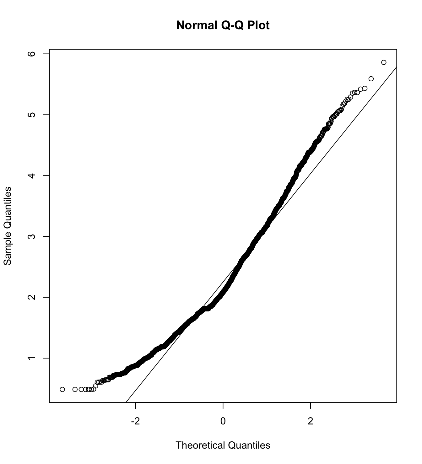
We first specify the factorial structure of the items, then fit models using a robust maximum likelihood estimator for the entire sample as well as for each country individually. The goodnes of fit indicators are shown.
# model
model_cfa <- ' gender_inquality =~ gen_in_1 + gen_in_2 + gen_in_3 + gen_in_4 + gen_in_5 + gen_in_6 '

# estimation
m5_cfa <- cfa(model = model_cfa,
              data = db_proc,
              estimator = "MLR",
              ordered = F,
              std.lv = F)

m5_cfa_arg <- cfa(model = model_cfa,
              data = subset(db_proc, country_residence_recoded == 1),
              estimator = "MLR",
              ordered = F,
              std.lv = F)

m5_cfa_cl <- cfa(model = model_cfa,
              data = subset(db_proc, country_residence_recoded == 3),
              estimator = "MLR",
              ordered = F,
              std.lv = F)

m5_cfa_col <- cfa(model = model_cfa,
              data = subset(db_proc, country_residence_recoded == 4),
              estimator = "MLR",
              ordered = F,
              std.lv = F)

m5_cfa_es <- cfa(model = model_cfa,
              data = subset(db_proc, country_residence_recoded == 9),
              estimator = "MLR",
              ordered = F,
              std.lv = F)

m5_cfa_mex <- cfa(model = model_cfa,
              data = subset(db_proc, country_residence_recoded == 13),
              estimator = "MLR",
              ordered = F,
std.lv = F) cfa_tab_fit(
models = list(m5_cfa, m5_cfa_arg, m5_cfa_cl, m5_cfa_col, m5_cfa_es, m5_cfa_mex),
country_names = c("Overall scores", "Argentina", "Chile", "Colombia", "Spain", "México")
)$fit_table| \(N\) | Estimator | \(\chi^2\) (df) | CFI | TLI | RMSEA 90% CI [Lower-Upper] | SRMR | AIC | |
|---|---|---|---|---|---|---|---|---|
| Overall scores | 4209 | ML | 104.751 (9) *** | 0.985 | 0.975 | 0.05 [0.042-0.059] | 0.022 | 97265.33 |
| Argentina | 807 | ML | 39.691 (9) *** | 0.975 | 0.958 | 0.065 [0.045-0.086] | 0.033 | 19036.01 |
| Chile | 883 | ML | 50.238 (9) *** | 0.965 | 0.941 | 0.072 [0.053-0.092] | 0.036 | 20337.77 |
| Colombia | 833 | ML | 28.297 (9) *** | 0.982 | 0.970 | 0.051 [0.03-0.072] | 0.027 | 19551.93 |
| Spain | 835 | ML | 46.197 (9) *** | 0.981 | 0.969 | 0.07 [0.051-0.091] | 0.028 | 18118.03 |
| México | 846 | ML | 21.14 (9) * | 0.990 | 0.984 | 0.04 [0.018-0.062] | 0.021 | 19692.44 |
5.2.3 Belief in sexism shift
The items to capture belief in sexism shift came from previous research from Zehnter et al. (2021). We translated four items from the original scale, adapting them to our context and objectives. These items are the ones that saturate the most in the scale across various studies.
Descriptive results
describe_kable(db_proc, c("shif_1", "shif_2", "shif_3"))| vars | n | mean | sd | median | trimmed | mad | min | max | range | skew | kurtosis | se | |
|---|---|---|---|---|---|---|---|---|---|---|---|---|---|
| shif_1 | 1 | 4209 | 3.507 | 1.994 | 4 | 3.384 | 2.965 | 1 | 7 | 6 | 0.211 | -1.123 | 0.031 |
| shif_2 | 2 | 4209 | 3.192 | 1.995 | 3 | 3.004 | 2.965 | 1 | 7 | 6 | 0.428 | -1.019 | 0.031 |
| shif_3 | 3 | 4209 | 3.286 | 2.112 | 3 | 3.107 | 2.965 | 1 | 7 | 6 | 0.371 | -1.213 | 0.033 |
wrap_elements(
    ~corrplot::corrplot(
      fit_correlations(db_proc, c("shif_1", "shif_2", "shif_3")),
      method = "color",
      type = "upper",
      col = colorRampPalette(c("#E16462", "white", "#0D0887"))(12),
      tl.pos = "lt",
      tl.col = "black",
      addrect = 2,
      rect.col = "black",
      addCoef.col = "white",
      cl.cex = 0.8,
      cl.align.text = 'l',
      number.cex = 1.1,
      na.label = "-",
      bg = "white"
    )
  ) + labs(caption = paste0(
    "Source: Authors calculation based on SOGEDI",
    " database (n=", nrow(db_proc), ")"
  ))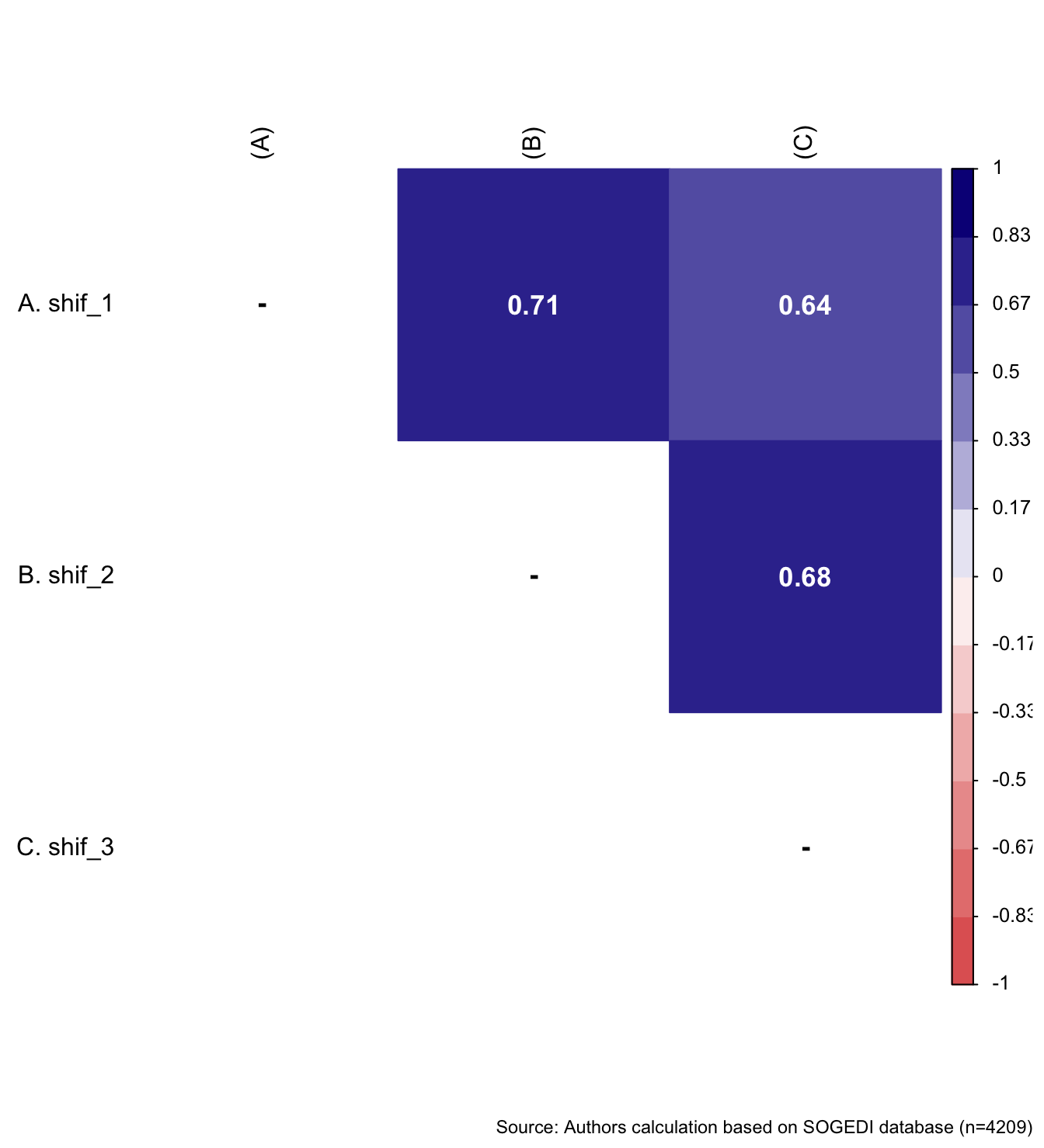
Reliability
mi_variable <- "shif"
result2 <- alphas(db_proc, c("shif_1", "shif_2", "shif_3"), mi_variable)

result2$raw_alpha
[1] 0.8612019result2$new_var_summary Min. 1st Qu. Median Mean 3rd Qu. Max.
1.000 1.667 3.333 3.328 4.667 7.000 Confirmatory factor analysis
Mardia’s test for evaluate multivariate normality.
mardia(db_proc[,c("shif_1", "shif_2", "shif_3")],
       na.rm = T, plot=T)
Call: mardia(x = db_proc[, c(“shif_1”, “shif_2”, “shif_3”)], na.rm = T, plot = T)
Mardia tests of multivariate skew and kurtosis Use describe(x) the to get univariate tests n.obs = 4209 num.vars = 3 b1p = 0.37 skew = 258.14 with probability <= 0.00000000000000000000000000000000000000000000000011 small sample skew = 258.42 with probability <= 0.000000000000000000000000000000000000000000000000092 b2p = 18.61 kurtosis = 21.39 with probability <= 0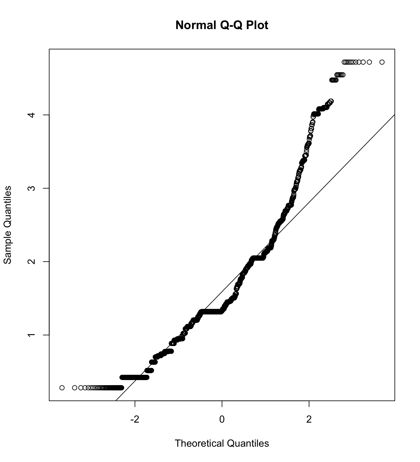
We first specify the factorial structure of the items, then fit models using a robust maximum likelihood estimator for the entire sample as well as for each country individually. The goodnes of fit indicators are shown.
# model
model_cfa <- ' shif_sexism =~ shif_1 + shif_2 + shif_3 '

# estimation
m6_cfa <- cfa(model = model_cfa,
              data = db_proc,
              estimator = "MLR",
              ordered = F,
              std.lv = F)

m6_cfa_arg <- cfa(model = model_cfa,
              data = subset(db_proc, country_residence_recoded == 1),
              estimator = "MLR",
              ordered = F,
              std.lv = F)

m6_cfa_cl <- cfa(model = model_cfa,
              data = subset(db_proc, country_residence_recoded == 3),
              estimator = "MLR",
              ordered = F,
              std.lv = F)

m6_cfa_col <- cfa(model = model_cfa,
              data = subset(db_proc, country_residence_recoded == 4),
              estimator = "MLR",
              ordered = F,
              std.lv = F)

m6_cfa_es <- cfa(model = model_cfa,
              data = subset(db_proc, country_residence_recoded == 9),
              estimator = "MLR",
              ordered = F,
              std.lv = F)

m6_cfa_mex <- cfa(model = model_cfa,
              data = subset(db_proc, country_residence_recoded == 13),
              estimator = "MLR",
              ordered = F,
std.lv = F) cfa_tab_fit(
models = list(m6_cfa, m6_cfa_arg, m6_cfa_cl, m6_cfa_col, m6_cfa_es, m6_cfa_mex),
country_names = c("Overall scores", "Argentina", "Chile", "Colombia", "Spain", "México")
)$fit_table| \(N\) | Estimator | \(\chi^2\) (df) | CFI | TLI | RMSEA 90% CI [Lower-Upper] | SRMR | AIC | |
|---|---|---|---|---|---|---|---|---|
| Overall scores | 4209 | ML | 0 (0) | 1 | 1 | 0 [0-0] | 0 | 47815.314 |
| Argentina | 807 | ML | 0 (0) | 1 | 1 | 0 [0-0] | 0 | 9215.297 |
| Chile | 883 | ML | 0 (0) | 1 | 1 | 0 [0-0] | 0 | 9970.867 |
| Colombia | 833 | ML | 0 (0) | 1 | 1 | 0 [0-0] | 0 | 9605.729 |
| Spain | 835 | ML | 0 (0) | 1 | 1 | 0 [0-0] | 0 | 8687.609 |
| México | 846 | ML | 0 (0) | 1 | 1 | 0 [0-0] | 0 | 9885.223 |
5.2.4 Feminism identification
The item to capture feminism identification came from previous research from Estevan-Reina et al. (2020). We translated the item from the original scale, adapting to our context and objectives.
Descriptive analysis
5.2.5 Gender inequality justification
The item to capture feminism identification came from previous research from Jost & Kay (2005). We translated the item from the original scale, adapting to our context and objectives.
5.2.6 Gender inequality collective action
The item to capture gender inequality collective action was created by the project team.
5.2.7 Perception of gender competition
The item to capture gender inequality collective action was created by the project team.
5.3 Block 3. Contacts and rates
5.3.1 Gendered poverty rates
The items to capture gender poverty rates was inspired by the research of Kuo et al. (2020).
describe_kable(db_proc, c("ge_ra_wo", "ge_ra_me"))| vars | n | mean | sd | median | trimmed | mad | min | max | range | skew | kurtosis | se | |
|---|---|---|---|---|---|---|---|---|---|---|---|---|---|
| ge_ra_wo | 1 | 4209 | 52.366 | 12.893 | 50 | 52.832 | 14.826 | 5 | 100 | 95 | -0.289 | 0.343 | 0.199 |
| ge_ra_me | 2 | 4209 | 47.634 | 12.893 | 50 | 47.168 | 14.826 | 0 | 95 | 95 | 0.289 | 0.343 | 0.199 |
5.3.2 Intergroup contacts: quantity of contacts
The variables used to capture this inter group contacts was derived from previous research from Vargas et al. (2023) and Vázquez et al. (2023). The wording of the items is based on the COES longitudinal survey, incorporating some supplementary information from Vargas et al. (2023) regarding the places where contact can occur.
describe_kable(db_proc, c("quan_pw", "quan_pm", "quan_rw", "quan_rm"))| vars | n | mean | sd | median | trimmed | mad | min | max | range | skew | kurtosis | se | |
|---|---|---|---|---|---|---|---|---|---|---|---|---|---|
| quan_pw | 1 | 4209 | 4.162 | 1.799 | 4 | 4.164 | 1.483 | 1 | 7 | 6 | 0.082 | -0.937 | 0.028 |
| quan_pm | 2 | 4209 | 4.166 | 1.824 | 4 | 4.175 | 1.483 | 1 | 7 | 6 | 0.063 | -0.978 | 0.028 |
| quan_rw | 3 | 4209 | 4.066 | 1.732 | 4 | 4.065 | 1.483 | 1 | 7 | 6 | -0.019 | -0.812 | 0.027 |
| quan_rm | 4 | 4209 | 4.096 | 1.762 | 4 | 4.105 | 1.483 | 1 | 7 | 6 | -0.054 | -0.876 | 0.027 |
5.3.3 Intergroup contacts: friendship
The variables used to capture this inter group friendship was developed by the project team.
describe_kable(db_proc, c("fri_pw", "fri_pm", "fri_rw", "fri_rm"))| vars | n | mean | sd | median | trimmed | mad | min | max | range | skew | kurtosis | se | |
|---|---|---|---|---|---|---|---|---|---|---|---|---|---|
| fri_pw | 1 | 4209 | 2.800 | 1.732 | 2 | 2.598 | 1.483 | 1 | 7 | 6 | 0.719 | -0.372 | 0.027 |
| fri_pm | 2 | 4209 | 2.790 | 1.737 | 2 | 2.581 | 1.483 | 1 | 7 | 6 | 0.730 | -0.364 | 0.027 |
| fri_rw | 3 | 4209 | 3.587 | 1.711 | 4 | 3.545 | 1.483 | 1 | 7 | 6 | 0.046 | -0.863 | 0.026 |
| fri_rm | 4 | 4209 | 3.601 | 1.749 | 4 | 3.555 | 1.483 | 1 | 7 | 6 | 0.066 | -0.901 | 0.027 |
5.3.4 Intergroup contacts: quality of contacts
The variables used to capture this inter group contacts was derived from previous research from Vázquez et al. (2023).
describe_kable(db_proc, c("qual_pw", "qual_pm", "qual_rw", "qual_rm"))| vars | n | mean | sd | median | trimmed | mad | min | max | range | skew | kurtosis | se | |
|---|---|---|---|---|---|---|---|---|---|---|---|---|---|
| qual_pw | 1 | 4209 | 4.671 | 1.378 | 4 | 4.679 | 1.483 | 1 | 7 | 6 | -0.044 | -0.185 | 0.021 |
| qual_pm | 2 | 4209 | 4.445 | 1.415 | 4 | 4.447 | 1.483 | 1 | 7 | 6 | -0.043 | -0.097 | 0.022 |
| qual_rw | 3 | 4209 | 4.174 | 1.410 | 4 | 4.187 | 1.483 | 1 | 7 | 6 | -0.052 | -0.083 | 0.022 |
| qual_rm | 4 | 4209 | 4.148 | 1.440 | 4 | 4.166 | 1.483 | 1 | 7 | 6 | -0.092 | -0.131 | 0.022 |
5.3.5 Perception of social mobility
For social mobility perceptions, we selected the items from the scale developed by Matamoros-Lima et al. (2023) that better suits our context of study having in mind the survey space limitations.
Descriptive results
describe_kable(db_proc, c("mobi_up_1", "mobi_up_2", "mobi_up_3", "mobi_down_1", "mobi_down_2", "mobi_down_3"))| vars | n | mean | sd | median | trimmed | mad | min | max | range | skew | kurtosis | se | |
|---|---|---|---|---|---|---|---|---|---|---|---|---|---|
| mobi_up_1 | 1 | 4209 | 4.285 | 1.525 | 4 | 4.321 | 1.483 | 1 | 7 | 6 | -0.222 | -0.367 | 0.024 |
| mobi_up_2 | 2 | 4209 | 3.941 | 1.531 | 4 | 3.966 | 1.483 | 1 | 7 | 6 | -0.130 | -0.378 | 0.024 |
| mobi_up_3 | 3 | 4209 | 4.365 | 1.545 | 4 | 4.421 | 1.483 | 1 | 7 | 6 | -0.332 | -0.270 | 0.024 |
| mobi_down_1 | 4 | 4209 | 4.133 | 1.663 | 4 | 4.126 | 1.483 | 1 | 7 | 6 | 0.020 | -0.672 | 0.026 |
| mobi_down_2 | 5 | 4209 | 3.772 | 1.593 | 4 | 3.740 | 1.483 | 1 | 7 | 6 | 0.157 | -0.495 | 0.025 |
| mobi_down_3 | 6 | 4209 | 3.491 | 1.557 | 3 | 3.431 | 1.483 | 1 | 7 | 6 | 0.268 | -0.418 | 0.024 |
wrap_elements(
    ~corrplot::corrplot(
      fit_correlations(db_proc, c("mobi_up_1", "mobi_up_2", "mobi_up_3", "mobi_down_1", "mobi_down_2", "mobi_down_3")),
      method = "color",
      type = "upper",
      col = colorRampPalette(c("#E16462", "white", "#0D0887"))(12),
      tl.pos = "lt",
      tl.col = "black",
      addrect = 2,
      rect.col = "black",
      addCoef.col = "white",
      cl.cex = 0.8,
      cl.align.text = 'l',
      number.cex = 1.1,
      na.label = "-",
      bg = "white"
    )
  ) + labs(caption = paste0(
    "Source: Authors calculation based on SOGEDI",
    " database (n=", nrow(db_proc), ")"
  ))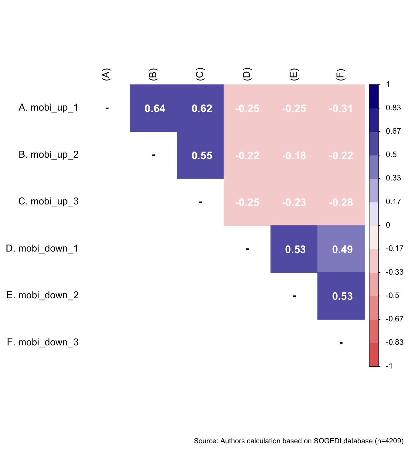
Reliability
mi_variable <- "ascenmobi"
result2 <- alphas(db_proc, c("mobi_up_1", "mobi_up_2", "mobi_up_3"), mi_variable)

result2$raw_alpha
[1] 0.8200618result2$new_var_summary Min. 1st Qu. Median Mean 3rd Qu. Max.
1.000 3.333 4.333 4.197 5.000 7.000 mi_variable <- "descenmobi"
result3 <- alphas(db_proc, c("mobi_down_1", "mobi_down_2", "mobi_down_3"), mi_variable)
result3$raw_alpha[1] 0.7613283result3$new_var_summary Min. 1st Qu. Median Mean 3rd Qu. Max.
1.000 3.000 3.667 3.799 4.667 7.000 Confirmatory factor analysis
Mardia’s test for evaluate multivariate normality.
mardia(db_proc[,c("mobi_up_1", "mobi_up_2", "mobi_up_3",
                  "mobi_down_1", "mobi_down_2", "mobi_down_3")],
       na.rm = T, plot=T)
Call: mardia(x = db_proc[, c(“mobi_up_1”, “mobi_up_2”, “mobi_up_3”, “mobi_down_1”, “mobi_down_2”, “mobi_down_3”)], na.rm = T, plot = T)
Mardia tests of multivariate skew and kurtosis Use describe(x) the to get univariate tests n.obs = 4209 num.vars = 6 b1p = 1.54 skew = 1082.29 with probability <= 0.00000000000000000000000000000000000000000000000000000000000000000000000000000000000000000000000000000000000000000000000000000000000000000000000000000000000000000000000000000000000000000000059 small sample skew = 1083.28 with probability <= 0.00000000000000000000000000000000000000000000000000000000000000000000000000000000000000000000000000000000000000000000000000000000000000000000000000000000000000000000000000000000000000000000037 b2p = 70.82 kurtosis = 75.56 with probability <= 0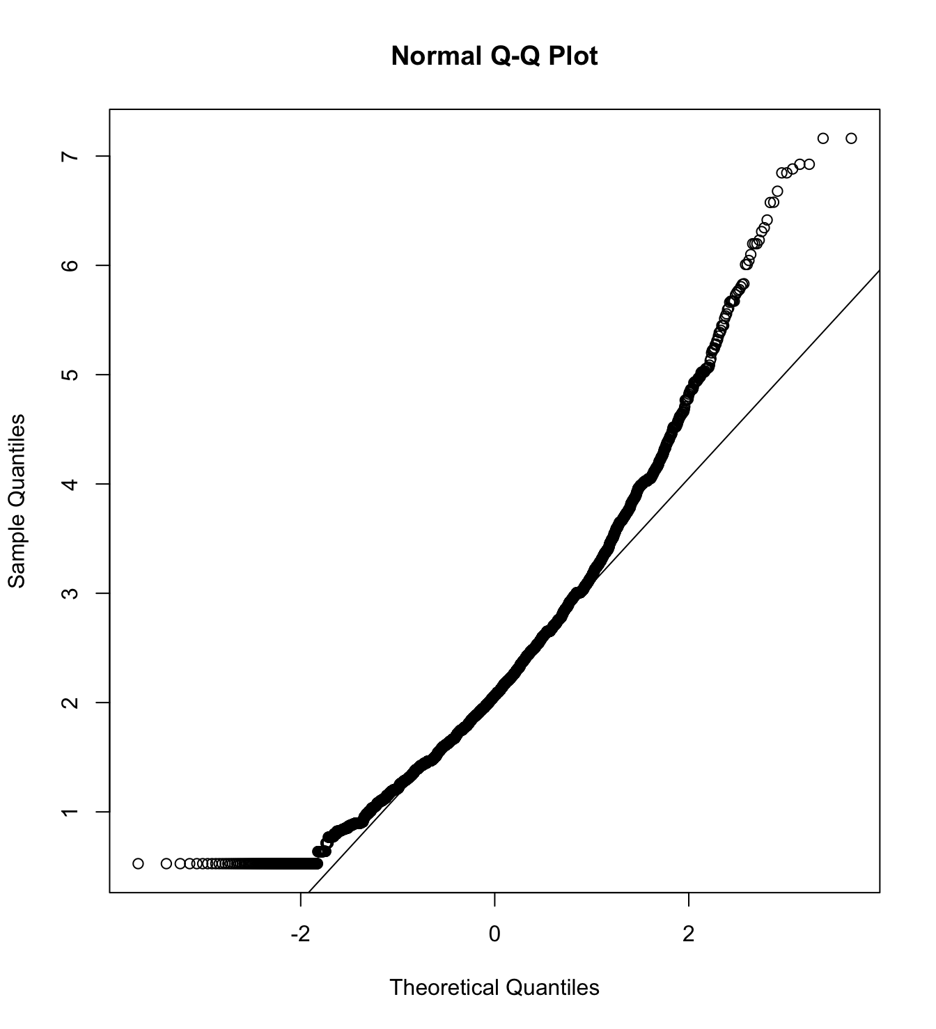
We first specify the factorial structure of the items, then fit models using a robust maximum likelihood estimator for the entire sample as well as for each country individually. The goodnes of fit indicators are shown.
# model
model_cfa <- '
  ascen_mobi =~ mobi_up_1 + mobi_up_2 + mobi_up_3
  descen_mobi =~ mobi_down_1 + mobi_down_2 + mobi_down_3
   '

# estimation
m7_cfa <- cfa(model = model_cfa,
              data = db_proc,
              estimator = "MLR",
              ordered = F,
              std.lv = F)

m7_cfa_arg <- cfa(model = model_cfa,
              data = subset(db_proc, country_residence_recoded == 1),
              estimator = "MLR",
              ordered = F,
              std.lv = F)

m7_cfa_cl <- cfa(model = model_cfa,
              data = subset(db_proc, country_residence_recoded == 3),
              estimator = "MLR",
              ordered = F,
              std.lv = F)

m7_cfa_col <- cfa(model = model_cfa,
              data = subset(db_proc, country_residence_recoded == 4),
              estimator = "MLR",
              ordered = F,
              std.lv = F)

m7_cfa_es <- cfa(model = model_cfa,
              data = subset(db_proc, country_residence_recoded == 9),
              estimator = "MLR",
              ordered = F,
              std.lv = F)

m7_cfa_mex <- cfa(model = model_cfa,
              data = subset(db_proc, country_residence_recoded == 13),
              estimator = "MLR",
              ordered = F,
std.lv = F) cfa_tab_fit(
models = list(m7_cfa, m7_cfa_arg, m7_cfa_cl, m7_cfa_col, m7_cfa_es, m7_cfa_mex),
country_names = c("Overall scores", "Argentina", "Chile", "Colombia", "Spain", "México")
)$fit_table| \(N\) | Estimator | \(\chi^2\) (df) | CFI | TLI | RMSEA 90% CI [Lower-Upper] | SRMR | AIC | |
|---|---|---|---|---|---|---|---|---|
| Overall scores | 4209 | ML | 75.006 (8) *** | 0.992 | 0.985 | 0.045 [0.036-0.054] | 0.022 | 86196.60 |
| Argentina | 807 | ML | 14.709 (8) . | 0.996 | 0.992 | 0.032 [0-0.058] | 0.022 | 16519.25 |
| Chile | 883 | ML | 32.329 (8) *** | 0.982 | 0.966 | 0.059 [0.038-0.08] | 0.038 | 17606.56 |
| Colombia | 833 | ML | 9.724 (8) | 0.999 | 0.998 | 0.016 [0-0.046] | 0.020 | 17128.96 |
| Spain | 835 | ML | 17.68 (8) * | 0.995 | 0.991 | 0.038 [0.013-0.062] | 0.020 | 15950.95 |
| México | 846 | ML | 39.068 (8) *** | 0.974 | 0.951 | 0.068 [0.047-0.09] | 0.034 | 17776.29 |
5.4 Block 4. Stereotype content model
5.4.1 Inmmorality
We included the immorality scale in an exploratory manner. The items are form the published article from Sánchez-Castelló et al. (2022).
Descriptive analysis
db_proc <- db_proc %>%
  mutate(condi_gender = if_else(condi_gender == 0, "Men", "Women"),
         condi_class = if_else(condi_class == 0, "Poor", "Rich")) %>%
  rowwise() %>%
  mutate(target = interaction(condi_class, condi_gender)) %>%
  ungroup()

db_rm <- subset(db_proc, target == "Rich.Men")
db_pm <- subset(db_proc, target == "Poor.Men")
db_rw <- subset(db_proc, target == "Rich.Women")
db_pw <- subset(db_proc, target == "Poor.Women")

bind_rows(
psych::describe(db_rm[,c("inm_1", "inm_2", "inm_3")]) %>%
    as_tibble() %>%
    mutate(target = "Rich Men")
,
psych::describe(db_pm[,c("inm_1", "inm_2", "inm_3")]) %>%
    as_tibble() %>%
    mutate(target = "Poor Men")
,
psych::describe(db_rw[,c("inm_1", "inm_2", "inm_3")]) %>%
    as_tibble() %>%
    mutate(target = "Rich Women")
,
psych::describe(db_pw[,c("inm_1", "inm_2", "inm_3")]) %>%
    as_tibble() %>%
    mutate(target = "Poor Women")
) %>%
  mutate(vars = paste0("inm_", vars)) %>%
  select(target, everything()) %>%
  group_by(target) %>%
  mutate(target = if_else(duplicated(target), NA, target)) %>%
kableExtra::kable(format = "markdown", digits = 3)| target | vars | n | mean | sd | median | trimmed | mad | min | max | range | skew | kurtosis | se |
|---|---|---|---|---|---|---|---|---|---|---|---|---|---|
| Rich Men | inm_1 | 1043 | 4.189 | 1.525 | 4 | 4.206 | 1.483 | 1 | 7 | 6 | -0.122 | -0.346 | 0.047 |
| inm_2 | 1043 | 3.940 | 1.480 | 4 | 3.925 | 1.483 | 1 | 7 | 6 | 0.054 | -0.268 | 0.046 | |
| inm_3 | 1043 | 4.095 | 1.570 | 4 | 4.117 | 1.483 | 1 | 7 | 6 | -0.127 | -0.428 | 0.049 | |
| Poor Men | inm_1 | 1058 | 3.806 | 1.481 | 4 | 3.811 | 1.483 | 1 | 7 | 6 | -0.057 | -0.489 | 0.046 |
| inm_2 | 1058 | 3.317 | 1.482 | 3 | 3.278 | 1.483 | 1 | 7 | 6 | 0.164 | -0.503 | 0.046 | |
| inm_3 | 1058 | 3.638 | 1.525 | 4 | 3.636 | 1.483 | 1 | 7 | 6 | 0.007 | -0.589 | 0.047 | |
| Rich Women | inm_1 | 1056 | 3.934 | 1.576 | 4 | 3.947 | 1.483 | 1 | 7 | 6 | -0.058 | -0.588 | 0.048 |
| inm_2 | 1056 | 3.689 | 1.569 | 4 | 3.676 | 1.483 | 1 | 7 | 6 | 0.082 | -0.520 | 0.048 | |
| inm_3 | 1056 | 3.751 | 1.674 | 4 | 3.723 | 1.483 | 1 | 7 | 6 | 0.109 | -0.678 | 0.052 | |
| Poor Women | inm_1 | 1052 | 3.396 | 1.471 | 4 | 3.381 | 1.483 | 1 | 7 | 6 | 0.104 | -0.639 | 0.045 |
| inm_2 | 1052 | 2.769 | 1.390 | 3 | 2.677 | 1.483 | 1 | 7 | 6 | 0.457 | -0.287 | 0.043 | |
| inm_3 | 1052 | 3.021 | 1.480 | 3 | 2.943 | 1.483 | 1 | 7 | 6 | 0.330 | -0.513 | 0.046 |
p1 <- wrap_elements(
    ~corrplot::corrplot(
      fit_correlations(db_rm, c("inm_1", "inm_2", "inm_3")),
      method = "color",
      type = "upper",
      col = colorRampPalette(c("#E16462", "white", "#0D0887"))(12),
      tl.pos = "lt",
      tl.col = "black",
      addrect = 2,
      rect.col = "black",
      addCoef.col = "white",
      cl.cex = 0.8,
      cl.align.text = 'l',
      number.cex = 1.1,
      na.label = "-",
      bg = "white"
    )
  ) + labs(title = "I. Rich Men")


p2 <- wrap_elements(
    ~corrplot::corrplot(
      fit_correlations(db_pm, c("inm_1", "inm_2", "inm_3")),
      method = "color",
      type = "upper",
      col = colorRampPalette(c("#E16462", "white", "#0D0887"))(12),
      tl.pos = "lt",
      tl.col = "black",
      addrect = 2,
      rect.col = "black",
      addCoef.col = "white",
      cl.cex = 0.8,
      cl.align.text = 'l',
      number.cex = 1.1,
      na.label = "-",
      bg = "white"
    )
  ) + labs(title = "II. Poor Men")

p3 <- wrap_elements(
    ~corrplot::corrplot(
      fit_correlations(db_rw, c("inm_1", "inm_2", "inm_3")),
      method = "color",
      type = "upper",
      col = colorRampPalette(c("#E16462", "white", "#0D0887"))(12),
      tl.pos = "lt",
      tl.col = "black",
      addrect = 2,
      rect.col = "black",
      addCoef.col = "white",
      cl.cex = 0.8,
      cl.align.text = 'l',
      number.cex = 1.1,
      na.label = "-",
      bg = "white"
    )
  ) + labs(title = "III. Rich Women")

p4 <- wrap_elements(
    ~corrplot::corrplot(
      fit_correlations(db_pw, c("inm_1", "inm_2", "inm_3")),
      method = "color",
      type = "upper",
      col = colorRampPalette(c("#E16462", "white", "#0D0887"))(12),
      tl.pos = "lt",
      tl.col = "black",
      addrect = 2,
      rect.col = "black",
      addCoef.col = "white",
      cl.cex = 0.8,
      cl.align.text = 'l',
      number.cex = 1.1,
      na.label = "-",
      bg = "white"
    )
  )+ labs(title = "VI. Poor Women")

a <- p1 + p2

b <- p3 + p4

a/b +
    plot_annotation(
      caption = paste0(
        "Source: Authors calculation based on SOGEDI",
        " database (n=", nrow(db_proc), ")"
      )
    )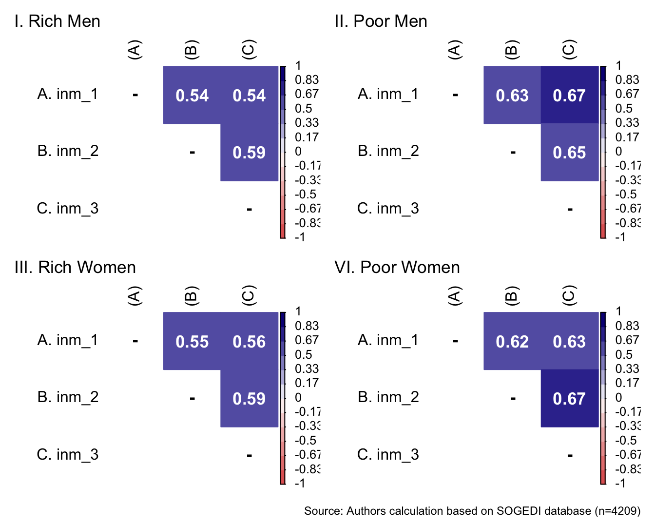
Reliability
mi_variable <- "inm"
result2 <- alphas(db_proc, c("inm_1", "inm_2", "inm_3"), mi_variable)

result2$raw_alpha
[1] 0.83072result2$new_var_summary Min. 1st Qu. Median Mean 3rd Qu. Max.
1.000 2.667 3.667 3.628 4.333 7.000 Confirmatory factor analysis
Mardia’s test for evaluate multivariate normality for each target.
mardia(db_rm[,c("inm_1", "inm_2", "inm_3")],
na.rm = T, plot=T) 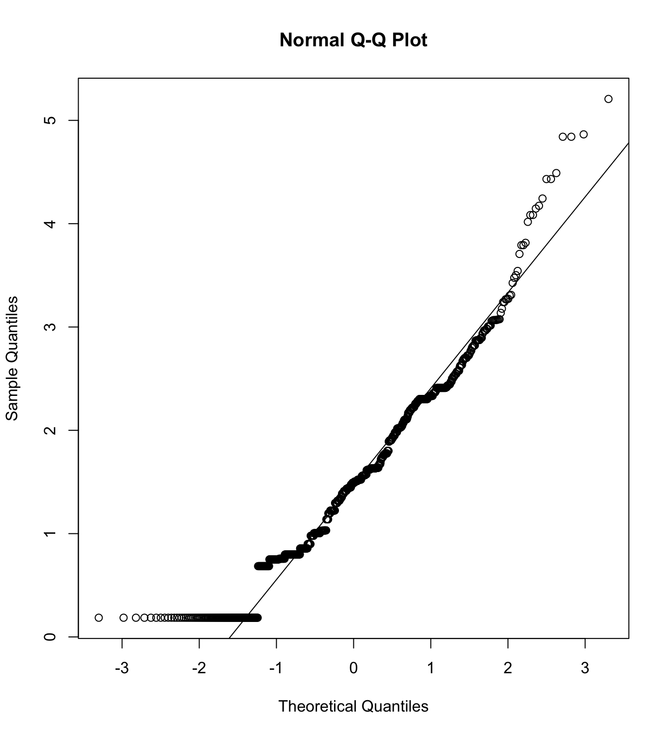 Call: mardia(x = db_rm[, c(“inm_1”, “inm_2”, “inm_3”)], na.rm = T, plot = T)
mardia(db_pm[,c("inm_1", "inm_2", "inm_3")],
na.rm = T, plot=T) 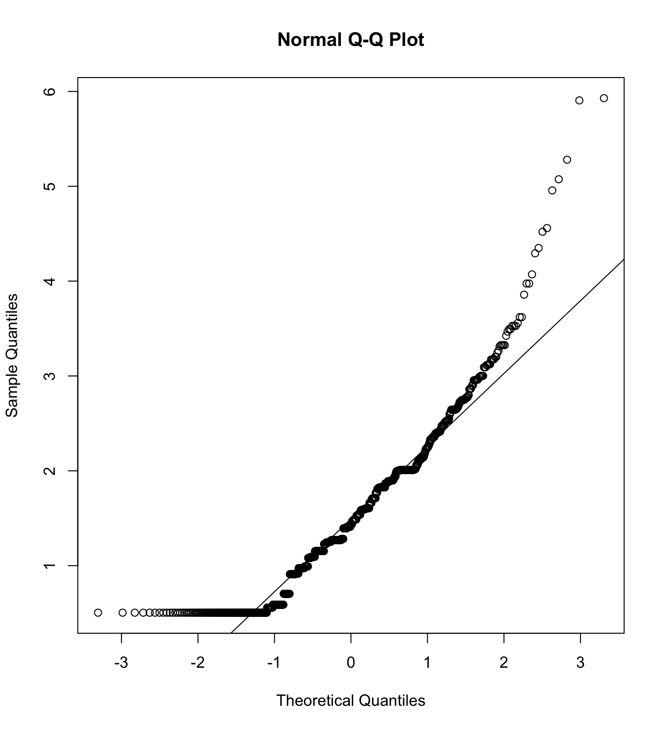 Call: mardia(x = db_pm[, c(“inm_1”, “inm_2”, “inm_3”)], na.rm = T, plot = T)
mardia(db_rw[,c("inm_1", "inm_2", "inm_3")],
na.rm = T, plot=T) 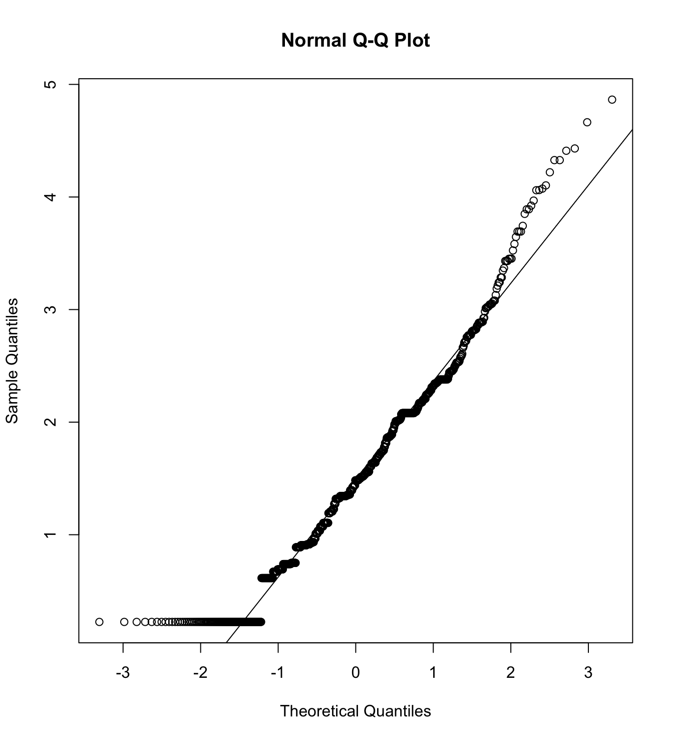 Call: mardia(x = db_rw[, c(“inm_1”, “inm_2”, “inm_3”)], na.rm = T, plot = T)
mardia(db_pw[,c("inm_1", "inm_2", "inm_3")],
na.rm = T, plot=T) 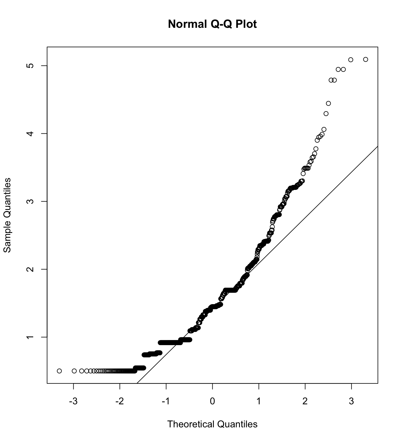 Call: mardia(x = db_pw[, c(“inm_1”, “inm_2”, “inm_3”)], na.rm = T, plot = T)
We first specify the factorial structure of the items, then fit models using a robust maximum likelihood estimator for the entire sample as well as for each country individually. The goodnes of fit indicators are shown.
# model
model_cfa <- '
  inmorality =~ inm_1 + inm_2 + inm_3
   '

# estimation
# overall
m8_cfa_rm <- cfa(model = model_cfa,
              data = subset(db_proc, target == "Rich.Men"),
              estimator = "MLR",
              ordered = F,
              std.lv = F)

m8_cfa_pm <- cfa(model = model_cfa,
              data = subset(db_proc, target == "Poor.Men"),
              estimator = "MLR",
              ordered = F,
              std.lv = F)

m8_cfa_rw <- cfa(model = model_cfa,
              data = subset(db_proc, target == "Rich.Women"),
              estimator = "MLR",
              ordered = F,
              std.lv = F)

m8_cfa_pw <- cfa(model = model_cfa,
              data = subset(db_proc, target == "Poor.Women"),
              estimator = "MLR",
              ordered = F,
              std.lv = F)

# per country
db_proc$group <- interaction(db_proc$natio_recoded, db_proc$target)

# argentina
m8_cfa_rm_arg <- cfa(model = model_cfa,
                 data = subset(db_proc, group == "1.Rich.Men"),
                 estimator = "MLR",
                 ordered = F,
                 std.lv = F)

m8_cfa_pm_arg <- cfa(model = model_cfa,
                 data = subset(db_proc, group == "1.Poor.Men"),
                 estimator = "MLR",
                 ordered = F,
                 std.lv = F)

m8_cfa_rw_arg <- cfa(model = model_cfa,
                 data = subset(db_proc, group == "1.Rich.Women"),
                 estimator = "MLR",
                 ordered = F,
                 std.lv = F)

m8_cfa_pw_arg <- cfa(model = model_cfa,
                 data = subset(db_proc, group == "1.Poor.Women"),
                 estimator = "MLR",
                 ordered = F,
                 std.lv = F)

# chile
m8_cfa_rm_cl <- cfa(model = model_cfa,
                     data = subset(db_proc, group == "3.Rich.Men"),
                     estimator = "MLR",
                     ordered = F,
                     std.lv = F)

m8_cfa_pm_cl <- cfa(model = model_cfa,
                     data = subset(db_proc, group == "3.Poor.Men"),
                     estimator = "MLR",
                     ordered = F,
                     std.lv = F)

m8_cfa_rw_cl <- cfa(model = model_cfa,
                     data = subset(db_proc, group == "3.Rich.Women"),
                     estimator = "MLR",
                     ordered = F,
                     std.lv = F)

m8_cfa_pw_cl <- cfa(model = model_cfa,
                     data = subset(db_proc, group == "3.Poor.Women"),
                     estimator = "MLR",
                     ordered = F,
                     std.lv = F)

# colombia
m8_cfa_rm_col <- cfa(model = model_cfa,
                     data = subset(db_proc, group == "4.Rich.Men"),
                     estimator = "MLR",
                     ordered = F,
                     std.lv = F)

m8_cfa_pm_col <- cfa(model = model_cfa,
                     data = subset(db_proc, group == "4.Poor.Men"),
                     estimator = "MLR",
                     ordered = F,
                     std.lv = F)

m8_cfa_rw_col <- cfa(model = model_cfa,
                     data = subset(db_proc, group == "4.Rich.Women"),
                     estimator = "MLR",
                     ordered = F,
                     std.lv = F)

m8_cfa_pw_col <- cfa(model = model_cfa,
                     data = subset(db_proc, group == "4.Poor.Women"),
                     estimator = "MLR",
                     ordered = F,
                     std.lv = F)

# españa
m8_cfa_rm_esp <- cfa(model = model_cfa,
                     data = subset(db_proc, group == "9.Rich.Men"),
                     estimator = "MLR",
                     ordered = F,
                     std.lv = F)

m8_cfa_pm_esp <- cfa(model = model_cfa,
                     data = subset(db_proc, group == "9.Poor.Men"),
                     estimator = "MLR",
                     ordered = F,
                     std.lv = F)

m8_cfa_rw_esp <- cfa(model = model_cfa,
                     data = subset(db_proc, group == "9.Rich.Women"),
                     estimator = "MLR",
                     ordered = F,
                     std.lv = F)

m8_cfa_pw_esp <- cfa(model = model_cfa,
                     data = subset(db_proc, group == "9.Poor.Women"),
                     estimator = "MLR",
                     ordered = F,
                     std.lv = F)

# mexico
m8_cfa_rm_mex <- cfa(model = model_cfa,
                     data = subset(db_proc, group == "13.Rich.Men"),
                     estimator = "MLR",
                     ordered = F,
                     std.lv = F)

m8_cfa_pm_mex <- cfa(model = model_cfa,
                     data = subset(db_proc, group == "13.Poor.Men"),
                     estimator = "MLR",
                     ordered = F,
                     std.lv = F)

m8_cfa_rw_mex <- cfa(model = model_cfa,
                     data = subset(db_proc, group == "13.Rich.Women"),
                     estimator = "MLR",
                     ordered = F,
                     std.lv = F)

m8_cfa_pw_mex <- cfa(model = model_cfa,
                     data = subset(db_proc, group == "13.Poor.Women"),
                     estimator = "MLR",
                     ordered = F,
                     std.lv = F)
colnames_fit <- c("","Target","$N$","Estimator","$\\chi^2$ (df)","CFI","TLI","RMSEA 90% CI [Lower-Upper]", "SRMR", "AIC")
bind_rows(
cfa_tab_fit(
models = list(m8_cfa_rm, m8_cfa_rm_arg, m8_cfa_rm_cl, m8_cfa_rm_col, m8_cfa_rm_esp, m8_cfa_rm_mex),
country_names = c("Overall scores", "Argentina", "Chile", "Colombia", "Spain", "México")
)$sum_fit %>%
mutate(target = "Rich Men")
,
cfa_tab_fit(
models = list(m8_cfa_pm, m8_cfa_pm_arg, m8_cfa_pm_cl, m8_cfa_pm_col, m8_cfa_pm_esp, m8_cfa_pm_mex),
country_names = c("Overall scores", "Argentina", "Chile", "Colombia", "Spain", "México")
)$sum_fit %>%
mutate(target = "Poor Men")
,
cfa_tab_fit(
models = list(m8_cfa_rw, m8_cfa_rw_arg, m8_cfa_rw_cl, m8_cfa_rw_col, m8_cfa_rw_esp, m8_cfa_rw_mex),
country_names = c("Overall scores", "Argentina", "Chile", "Colombia", "Spain", "México")
)$sum_fit %>%
mutate(target = "Rich Women")
,
cfa_tab_fit(
models = list(m8_cfa_pw, m8_cfa_pw_arg, m8_cfa_pw_cl, m8_cfa_pw_col, m8_cfa_pw_esp, m8_cfa_pw_mex),
country_names = c("Overall scores", "Argentina", "Chile", "Colombia", "Spain", "México")
)$sum_fit %>%
mutate(target = "Poor Women")
) %>%
select(country, target, everything()) %>%
mutate(country = factor(country, levels = c("Overall scores", "Argentina", "Chile", "Colombia", "Spain", "México"))) %>%
group_by(country) %>%
arrange(country) %>%
mutate(country = if_else(duplicated(country), NA, country)) %>%
kableExtra::kable(
format = "markdown",
digits = 3,
booktabs = TRUE,
col.names = colnames_fit,
caption = NULL
) %>%
kableExtra::kable_styling(
full_width = TRUE,
font_size = 11,
latex_options = "HOLD_position",
bootstrap_options = c("striped", "bordered")
) %>%
kableExtra::collapse_rows(columns = 1)| Target | \(N\) | Estimator | \(\chi^2\) (df) | CFI | TLI | RMSEA 90% CI [Lower-Upper] | SRMR | AIC | |
|---|---|---|---|---|---|---|---|---|---|
| Overall scores | Rich Men | 1043 | ML | 0 (0) | 1 | 1 | 0 [0-0] | 0 | 10611.363 |
| Poor Men | 1058 | ML | 0 (0) | 1 | 1 | 0 [0-0] | 0 | 10226.111 | |
| Rich Women | 1056 | ML | 0 (0) | 1 | 1 | 0 [0-0] | 0 | 11025.728 | |
| Poor Women | 1052 | ML | 0 (0) | 1 | 1 | 0 [0-0] | 0 | 10001.641 | |
| Argentina | Rich Men | 216 | ML | 0 (0) | 1 | 1 | 0 [0-0] | 0 | 2201.534 |
| Poor Men | 219 | ML | 0 (0) | 1 | 1 | 0 [0-0] | 0 | 2152.203 | |
| Rich Women | 207 | ML | 0 (0) | 1 | 1 | 0 [0-0] | 0 | 2180.033 | |
| Poor Women | 215 | ML | 0 (0) | 1 | 1 | 0 [0-0] | 0 | 2033.150 | |
| Chile | Rich Men | 217 | ML | 0 (0) | 1 | 1 | 0 [0-0] | 0 | 2221.275 |
| Poor Men | 215 | ML | 0 (0) | 1 | 1 | 0 [0-0] | 0 | 2058.520 | |
| Rich Women | 223 | ML | 0 (0) | 1 | 1 | 0 [0-0] | 0 | 2373.823 | |
| Poor Women | 205 | ML | 0 (0) | 1 | 1 | 0 [0-0] | 0 | 2032.958 | |
| Colombia | Rich Men | 206 | ML | 0 (0) | 1 | 1 | 0 [0-0] | 0 | 2096.875 |
| Poor Men | 214 | ML | 0 (0) | 1 | 1 | 0 [0-0] | 0 | 2103.545 | |
| Rich Women | 199 | ML | 0 (0) | 1 | 1 | 0 [0-0] | 0 | 2052.773 | |
| Poor Women | 205 | ML | 0 (0) | 1 | 1 | 0 [0-0] | 0 | 2017.228 | |
| Spain | Rich Men | 195 | ML | 0 (0) | 1 | 1 | 0 [0-0] | 0 | 1918.207 |
| Poor Men | 213 | ML | 0 (0) | 1 | 1 | 0 [0-0] | 0 | 1919.257 | |
| Rich Women | 212 | ML | 0 (0) | 1 | 1 | 0 [0-0] | 0 | 2088.505 | |
| Poor Women | 211 | ML | 0 (0) | 1 | 1 | 0 [0-0] | 0 | 1808.743 | |
| México | Rich Men | 209 | ML | 0 (0) | 1 | 1 | 0 [0-0] | 0 | 2176.784 |
| Poor Men | 197 | ML | 0 (0) | 1 | 1 | 0 [0-0] | 0 | 1950.643 | |
| Rich Women | 215 | ML | 0 (0) | 1 | 1 | 0 [0-0] | 0 | 2302.096 | |
| Poor Women | 216 | ML | 0 (0) | 1 | 1 | 0 [0-0] | 0 | 2041.889 |
5.4.2 Morality
We included the immorality scale in an exploratory manner. The items are form the published article from Sánchez-Castelló et al. (2022).
Descriptive analysis
bind_rows(
psych::describe(db_rm[,c("mor_1", "mor_2", "mor_3")]) %>%
    as_tibble() %>%
    mutate(target = "Rich Men")
,
psych::describe(db_pm[,c("mor_1", "mor_2", "mor_3")]) %>%
    as_tibble() %>%
    mutate(target = "Poor Men")
,
psych::describe(db_rw[,c("mor_1", "mor_2", "mor_3")]) %>%
    as_tibble() %>%
    mutate(target = "Rich Women")
,
psych::describe(db_pw[,c("mor_1", "mor_2", "mor_3")]) %>%
    as_tibble() %>%
    mutate(target = "Poor Women")
) %>%
  mutate(vars = paste0("mor_", vars)) %>%
  select(target, everything()) %>%
  group_by(target) %>%
  mutate(target = if_else(duplicated(target), NA, target)) %>%
kableExtra::kable(format = "markdown", digits = 3)| target | vars | n | mean | sd | median | trimmed | mad | min | max | range | skew | kurtosis | se |
|---|---|---|---|---|---|---|---|---|---|---|---|---|---|
| Rich Men | mor_1 | 1043 | 3.382 | 1.357 | 4 | 3.389 | 1.483 | 1 | 7 | 6 | 0.035 | -0.261 | 0.042 |
| mor_2 | 1043 | 3.555 | 1.389 | 4 | 3.576 | 1.483 | 1 | 7 | 6 | -0.066 | -0.181 | 0.043 | |
| mor_3 | 1043 | 3.354 | 1.367 | 3 | 3.349 | 1.483 | 1 | 7 | 6 | 0.107 | -0.117 | 0.042 | |
| Poor Men | mor_1 | 1058 | 4.250 | 1.367 | 4 | 4.244 | 1.483 | 1 | 7 | 6 | 0.048 | 0.084 | 0.042 |
| mor_2 | 1058 | 4.096 | 1.389 | 4 | 4.087 | 1.483 | 1 | 7 | 6 | 0.080 | -0.075 | 0.043 | |
| mor_3 | 1058 | 4.082 | 1.350 | 4 | 4.085 | 1.483 | 1 | 7 | 6 | 0.026 | 0.118 | 0.041 | |
| Rich Women | mor_1 | 1056 | 3.843 | 1.402 | 4 | 3.852 | 1.483 | 1 | 7 | 6 | -0.070 | -0.028 | 0.043 |
| mor_2 | 1056 | 3.876 | 1.406 | 4 | 3.887 | 1.483 | 1 | 7 | 6 | -0.096 | -0.053 | 0.043 | |
| mor_3 | 1056 | 3.728 | 1.431 | 4 | 3.719 | 1.483 | 1 | 7 | 6 | 0.031 | -0.113 | 0.044 | |
| Poor Women | mor_1 | 1052 | 4.667 | 1.310 | 4 | 4.650 | 1.483 | 1 | 7 | 6 | -0.007 | -0.210 | 0.040 |
| mor_2 | 1052 | 4.581 | 1.377 | 4 | 4.571 | 1.483 | 1 | 7 | 6 | -0.011 | -0.246 | 0.042 | |
| mor_3 | 1052 | 4.573 | 1.321 | 4 | 4.555 | 1.483 | 1 | 7 | 6 | -0.014 | -0.194 | 0.041 |
p1 <- wrap_elements(
    ~corrplot::corrplot(
      fit_correlations(db_rm, c("mor_1", "mor_2", "mor_3")),
      method = "color",
      type = "upper",
      col = colorRampPalette(c("#E16462", "white", "#0D0887"))(12),
      tl.pos = "lt",
      tl.col = "black",
      addrect = 2,
      rect.col = "black",
      addCoef.col = "white",
      cl.cex = 0.8,
      cl.align.text = 'l',
      number.cex = 1.1,
      na.label = "-",
      bg = "white"
    )
  ) + labs(title = "I. Rich Men")


p2 <- wrap_elements(
    ~corrplot::corrplot(
      fit_correlations(db_pm, c("mor_1", "mor_2", "mor_3")),
      method = "color",
      type = "upper",
      col = colorRampPalette(c("#E16462", "white", "#0D0887"))(12),
      tl.pos = "lt",
      tl.col = "black",
      addrect = 2,
      rect.col = "black",
      addCoef.col = "white",
      cl.cex = 0.8,
      cl.align.text = 'l',
      number.cex = 1.1,
      na.label = "-",
      bg = "white"
    )
  ) + labs(title = "II. Poor Men")

p3 <- wrap_elements(
    ~corrplot::corrplot(
      fit_correlations(db_rw, c("mor_1", "mor_2", "mor_3")),
      method = "color",
      type = "upper",
      col = colorRampPalette(c("#E16462", "white", "#0D0887"))(12),
      tl.pos = "lt",
      tl.col = "black",
      addrect = 2,
      rect.col = "black",
      addCoef.col = "white",
      cl.cex = 0.8,
      cl.align.text = 'l',
      number.cex = 1.1,
      na.label = "-",
      bg = "white"
    )
  ) + labs(title = "III. Rich Women")

p4 <- wrap_elements(
    ~corrplot::corrplot(
      fit_correlations(db_pw, c("mor_1", "mor_2", "mor_3")),
      method = "color",
      type = "upper",
      col = colorRampPalette(c("#E16462", "white", "#0D0887"))(12),
      tl.pos = "lt",
      tl.col = "black",
      addrect = 2,
      rect.col = "black",
      addCoef.col = "white",
      cl.cex = 0.8,
      cl.align.text = 'l',
      number.cex = 1.1,
      na.label = "-",
      bg = "white"
    )
  )+ labs(title = "VI. Poor Women")

a <- p1 + p2

b <- p3 + p4

a/b +
    plot_annotation(
      caption = paste0(
        "Source: Authors calculation based on SOGEDI",
        " database (n=", nrow(db_proc), ")"
      )
    )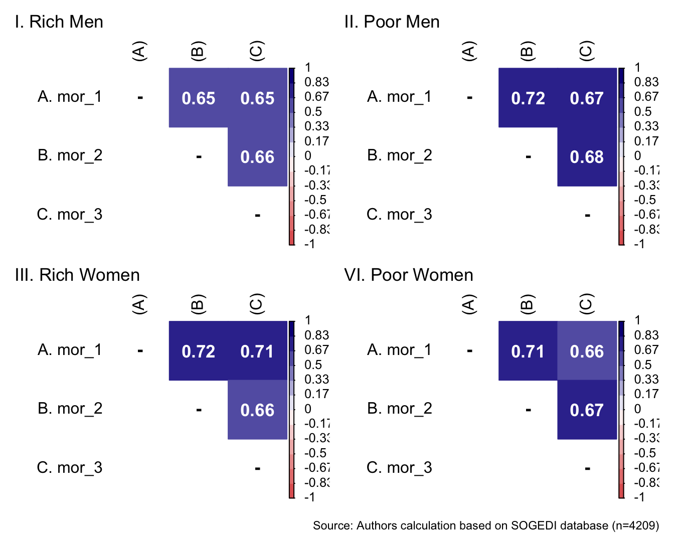
Reliability
mi_variable <- "mor"
result2 <- alphas(db_proc, c("mor_1", "mor_2", "mor_3"), mi_variable)

result2$raw_alpha
[1] 0.8784209result2$new_var_summary Min. 1st Qu. Median Mean 3rd Qu. Max.
1.000 3.333 4.000 4.000 4.667 7.000 Confirmatory factor analysis
Mardia’s test for evaluate multivariate normality for each target.
mardia(db_rm[,c("mor_1", "mor_2", "mor_3")],
       na.rm = T, plot=T)
Call: mardia(x = db_rm[, c(“mor_1”, “mor_2”, “mor_3”)], na.rm = T, plot = T)
Mardia tests of multivariate skew and kurtosis Use describe(x) the to get univariate tests n.obs = 1043 num.vars = 3 b1p = 0.27 skew = 46.46 with probability <= 0.0000012 small sample skew = 46.66 with probability <= 0.0000011 b2p = 23.23 kurtosis = 24.25 with probability <= 0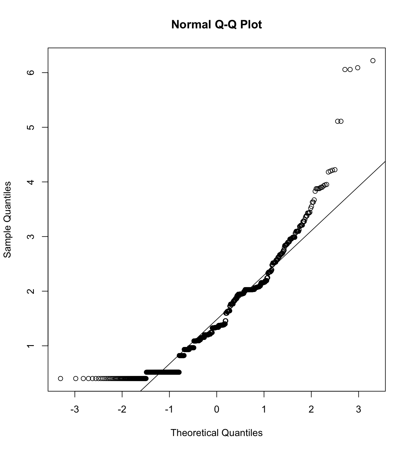
mardia(db_pm[,c("mor_1", "mor_2", "mor_3")],
       na.rm = T, plot=T)
Call: mardia(x = db_pm[, c(“mor_1”, “mor_2”, “mor_3”)], na.rm = T, plot = T)
Mardia tests of multivariate skew and kurtosis Use describe(x) the to get univariate tests n.obs = 1058 num.vars = 3 b1p = 0.72 skew = 127.47 with probability <= 0.00000000000000000000015 small sample skew = 128.01 with probability <= 0.00000000000000000000012 b2p = 26.15 kurtosis = 33.1 with probability <= 0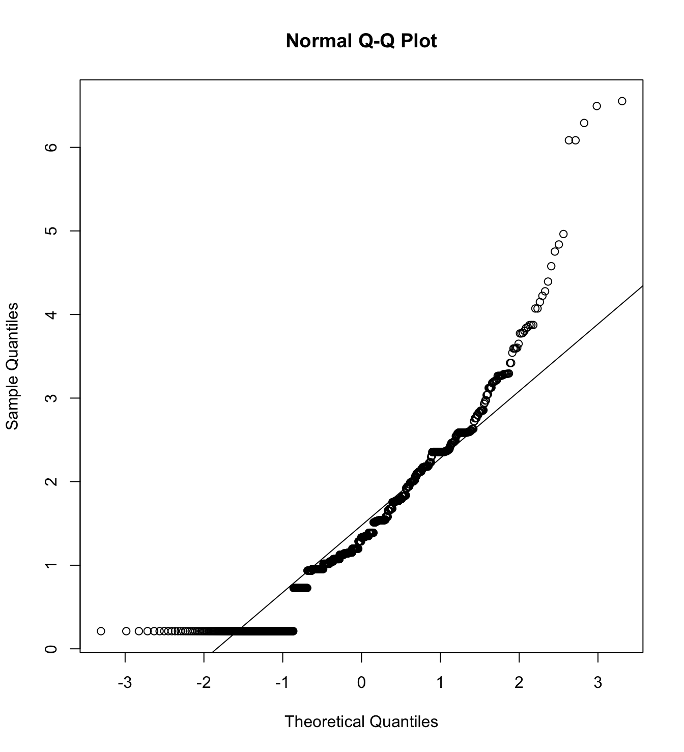
mardia(db_rw[,c("mor_1", "mor_2", "mor_3")],
       na.rm = T, plot=T)
Call: mardia(x = db_rw[, c(“mor_1”, “mor_2”, “mor_3”)], na.rm = T, plot = T)
Mardia tests of multivariate skew and kurtosis Use describe(x) the to get univariate tests n.obs = 1056 num.vars = 3 b1p = 0.06 skew = 11.1 with probability <= 0.35 small sample skew = 11.15 with probability <= 0.35 b2p = 23.08 kurtosis = 23.96 with probability <= 0
mardia(db_pw[,c("mor_1", "mor_2", "mor_3")],
       na.rm = T, plot=T)
Call: mardia(x = db_pw[, c(“mor_1”, “mor_2”, “mor_3”)], na.rm = T, plot = T)
Mardia tests of multivariate skew and kurtosis Use describe(x) the to get univariate tests n.obs = 1052 num.vars = 3 b1p = 0.18 skew = 31.33 with probability <= 0.00052 small sample skew = 31.46 with probability <= 0.00049 b2p = 21.73 kurtosis = 19.93 with probability <= 0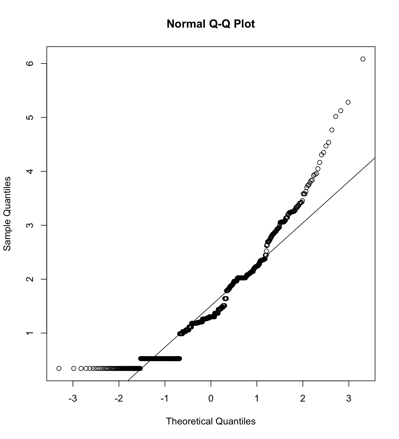
We first specify the factorial structure of the items, then fit models using a robust maximum likelihood estimator for the entire sample as well as for each country individually. The goodnes of fit indicators are shown.
# model
model_cfa <- '
  morality =~ mor_1 + mor_2 + mor_3
   '

# estimation
# overall
m9_cfa_rm <- cfa(model = model_cfa,
              data = subset(db_proc, target == "Rich.Men"),
              estimator = "MLR",
              ordered = F,
              std.lv = F)

m9_cfa_pm <- cfa(model = model_cfa,
              data = subset(db_proc, target == "Poor.Men"),
              estimator = "MLR",
              ordered = F,
              std.lv = F)

m9_cfa_rw <- cfa(model = model_cfa,
              data = subset(db_proc, target == "Rich.Women"),
              estimator = "MLR",
              ordered = F,
              std.lv = F)

m9_cfa_pw <- cfa(model = model_cfa,
              data = subset(db_proc, target == "Poor.Women"),
              estimator = "MLR",
              ordered = F,
              std.lv = F)


# argentina
m9_cfa_rm_arg <- cfa(model = model_cfa,
                 data = subset(db_proc, group == "1.Rich.Men"),
                 estimator = "MLR",
                 ordered = F,
                 std.lv = F)

m9_cfa_pm_arg <- cfa(model = model_cfa,
                 data = subset(db_proc, group == "1.Poor.Men"),
                 estimator = "MLR",
                 ordered = F,
                 std.lv = F)

m9_cfa_rw_arg <- cfa(model = model_cfa,
                 data = subset(db_proc, group == "1.Rich.Women"),
                 estimator = "MLR",
                 ordered = F,
                 std.lv = F)

m9_cfa_pw_arg <- cfa(model = model_cfa,
                 data = subset(db_proc, group == "1.Poor.Women"),
                 estimator = "MLR",
                 ordered = F,
                 std.lv = F)

# chile
m9_cfa_rm_cl <- cfa(model = model_cfa,
                     data = subset(db_proc, group == "3.Rich.Men"),
                     estimator = "MLR",
                     ordered = F,
                     std.lv = F)

m9_cfa_pm_cl <- cfa(model = model_cfa,
                     data = subset(db_proc, group == "3.Poor.Men"),
                     estimator = "MLR",
                     ordered = F,
                     std.lv = F)

m9_cfa_rw_cl <- cfa(model = model_cfa,
                     data = subset(db_proc, group == "3.Rich.Women"),
                     estimator = "MLR",
                     ordered = F,
                     std.lv = F)

m9_cfa_pw_cl <- cfa(model = model_cfa,
                     data = subset(db_proc, group == "3.Poor.Women"),
                     estimator = "MLR",
                     ordered = F,
                     std.lv = F)

# colombia
m9_cfa_rm_col <- cfa(model = model_cfa,
                     data = subset(db_proc, group == "4.Rich.Men"),
                     estimator = "MLR",
                     ordered = F,
                     std.lv = F)

m9_cfa_pm_col <- cfa(model = model_cfa,
                     data = subset(db_proc, group == "4.Poor.Men"),
                     estimator = "MLR",
                     ordered = F,
                     std.lv = F)

m9_cfa_rw_col <- cfa(model = model_cfa,
                     data = subset(db_proc, group == "4.Rich.Women"),
                     estimator = "MLR",
                     ordered = F,
                     std.lv = F)

m9_cfa_pw_col <- cfa(model = model_cfa,
                     data = subset(db_proc, group == "4.Poor.Women"),
                     estimator = "MLR",
                     ordered = F,
                     std.lv = F)

# españa
m9_cfa_rm_esp <- cfa(model = model_cfa,
                     data = subset(db_proc, group == "9.Rich.Men"),
                     estimator = "MLR",
                     ordered = F,
                     std.lv = F)

m9_cfa_pm_esp <- cfa(model = model_cfa,
                     data = subset(db_proc, group == "9.Poor.Men"),
                     estimator = "MLR",
                     ordered = F,
                     std.lv = F)

m9_cfa_rw_esp <- cfa(model = model_cfa,
                     data = subset(db_proc, group == "9.Rich.Women"),
                     estimator = "MLR",
                     ordered = F,
                     std.lv = F)

m9_cfa_pw_esp <- cfa(model = model_cfa,
                     data = subset(db_proc, group == "9.Poor.Women"),
                     estimator = "MLR",
                     ordered = F,
                     std.lv = F)

# mexico
m9_cfa_rm_mex <- cfa(model = model_cfa,
                     data = subset(db_proc, group == "13.Rich.Men"),
                     estimator = "MLR",
                     ordered = F,
                     std.lv = F)

m9_cfa_pm_mex <- cfa(model = model_cfa,
                     data = subset(db_proc, group == "13.Poor.Men"),
                     estimator = "MLR",
                     ordered = F,
                     std.lv = F)

m9_cfa_rw_mex <- cfa(model = model_cfa,
                     data = subset(db_proc, group == "13.Rich.Women"),
                     estimator = "MLR",
                     ordered = F,
                     std.lv = F)

m9_cfa_pw_mex <- cfa(model = model_cfa,
                     data = subset(db_proc, group == "13.Poor.Women"),
                     estimator = "MLR",
                     ordered = F,
                     std.lv = F)
colnames_fit <- c("","Target","$N$","Estimator","$\\chi^2$ (df)","CFI","TLI","RMSEA 90% CI [Lower-Upper]", "SRMR", "AIC")
bind_rows(
cfa_tab_fit(
models = list(m9_cfa_rm, m9_cfa_rm_arg, m9_cfa_rm_cl, m9_cfa_rm_col, m9_cfa_rm_esp, m9_cfa_rm_mex),
country_names = c("Overall scores", "Argentina", "Chile", "Colombia", "Spain", "México")
)$sum_fit %>%
mutate(target = "Rich Men")
,
cfa_tab_fit(
models = list(m9_cfa_pm, m9_cfa_pm_arg, m9_cfa_pm_cl, m9_cfa_pm_col, m9_cfa_pm_esp, m9_cfa_pm_mex),
country_names = c("Overall scores", "Argentina", "Chile", "Colombia", "Spain", "México")
)$sum_fit %>%
mutate(target = "Poor Men")
,
cfa_tab_fit(
models = list(m9_cfa_rw, m9_cfa_rw_arg, m9_cfa_rw_cl, m9_cfa_rw_col, m9_cfa_rw_esp, m9_cfa_rw_mex),
country_names = c("Overall scores", "Argentina", "Chile", "Colombia", "Spain", "México")
)$sum_fit %>%
mutate(target = "Rich Women")
,
cfa_tab_fit(
models = list(m9_cfa_pw, m9_cfa_pw_arg, m9_cfa_pw_cl, m9_cfa_pw_col, m9_cfa_pw_esp, m9_cfa_pw_mex),
country_names = c("Overall scores", "Argentina", "Chile", "Colombia", "Spain", "México")
)$sum_fit %>%
mutate(target = "Poor Women")
) %>%
select(country, target, everything()) %>%
mutate(country = factor(country, levels = c("Overall scores", "Argentina", "Chile", "Colombia", "Spain", "México"))) %>%
group_by(country) %>%
arrange(country) %>%
mutate(country = if_else(duplicated(country), NA, country)) %>%
kableExtra::kable(
format = "markdown",
digits = 3,
booktabs = TRUE,
col.names = colnames_fit,
caption = NULL
) %>%
kableExtra::kable_styling(
full_width = TRUE,
font_size = 11,
latex_options = "HOLD_position",
bootstrap_options = c("striped", "bordered")
) %>%
kableExtra::collapse_rows(columns = 1)| Target | \(N\) | Estimator | \(\chi^2\) (df) | CFI | TLI | RMSEA 90% CI [Lower-Upper] | SRMR | AIC | |
|---|---|---|---|---|---|---|---|---|---|
| Overall scores | Rich Men | 1043 | ML | 0 (0) | 1 | 1 | 0 [0-0] | 0 | 9540.692 |
| Poor Men | 1058 | ML | 0 (0) | 1 | 1 | 0 [0-0] | 0 | 9440.719 | |
| Rich Women | 1056 | ML | 0 (0) | 1 | 1 | 0 [0-0] | 0 | 9566.324 | |
| Poor Women | 1052 | ML | 0 (0) | 1 | 1 | 0 [0-0] | 0 | 9294.452 | |
| Argentina | Rich Men | 216 | ML | 0 (0) | 1 | 1 | 0 [0-0] | 0 | 2052.651 |
| Poor Men | 219 | ML | 0 (0) | 1 | 1 | 0 [0-0] | 0 | 1947.442 | |
| Rich Women | 207 | ML | 0 (0) | 1 | 1 | 0 [0-0] | 0 | 1818.548 | |
| Poor Women | 215 | ML | 0 (0) | 1 | 1 | 0 [0-0] | 0 | 1884.272 | |
| Chile | Rich Men | 217 | ML | 0 (0) | 1 | 1 | 0 [0-0] | 0 | 1946.342 |
| Poor Men | 215 | ML | 0 (0) | 1 | 1 | 0 [0-0] | 0 | 1912.601 | |
| Rich Women | 223 | ML | 0 (0) | 1 | 1 | 0 [0-0] | 0 | 2071.733 | |
| Poor Women | 205 | ML | 0 (0) | 1 | 1 | 0 [0-0] | 0 | 1794.739 | |
| Colombia | Rich Men | 206 | ML | 0 (0) | 1 | 1 | 0 [0-0] | 0 | 1929.650 |
| Poor Men | 214 | ML | 0 (0) | 1 | 1 | 0 [0-0] | 0 | 2049.164 | |
| Rich Women | 199 | ML | 0 (0) | 1 | 1 | 0 [0-0] | 0 | 1817.104 | |
| Poor Women | 205 | ML | 0 (0) | 1 | 1 | 0 [0-0] | 0 | 1901.407 | |
| Spain | Rich Men | 195 | ML | 0 (0) | 1 | 1 | 0 [0-0] | 0 | 1533.123 |
| Poor Men | 213 | ML | 0 (0) | 1 | 1 | 0 [0-0] | 0 | 1615.871 | |
| Rich Women | 212 | ML | 0 (0) | 1 | 1 | 0 [0-0] | 0 | 1680.451 | |
| Poor Women | 211 | ML | 0 (0) | 1 | 1 | 0 [0-0] | 0 | 1751.336 | |
| México | Rich Men | 209 | ML | 0 (0) | 1 | 1 | 0 [0-0] | 0 | 2003.526 |
| Poor Men | 197 | ML | 0 (0) | 1 | 1 | 0 [0-0] | 0 | 1817.122 | |
| Rich Women | 215 | ML | 0 (0) | 1 | 1 | 0 [0-0] | 0 | 2083.032 | |
| Poor Women | 216 | ML | 0 (0) | 1 | 1 | 0 [0-0] | 0 | 1919.010 |
5.4.3 Warmth
We included the immorality scale in an exploratory manner. The items are form the published article from Sánchez-Castelló et al. (2022).
Descriptive analysis
bind_rows(
psych::describe(db_rm[,c("war_1", "war_2", "war_3")]) %>%
    as_tibble() %>%
    mutate(target = "Rich Men")
,
psych::describe(db_pm[,c("war_1", "war_2", "war_3")]) %>%
    as_tibble() %>%
    mutate(target = "Poor Men")
,
psych::describe(db_rw[,c("war_1", "war_2", "war_3")]) %>%
    as_tibble() %>%
    mutate(target = "Rich Women")
,
psych::describe(db_pw[,c("war_1", "war_2", "war_3")]) %>%
    as_tibble() %>%
    mutate(target = "Poor Women")
) %>%
  mutate(vars = paste0("war_", vars)) %>%
  select(target, everything()) %>%
  group_by(target) %>%
  mutate(target = if_else(duplicated(target), NA, target)) %>%
kableExtra::kable(format = "markdown", digits = 3)| target | vars | n | mean | sd | median | trimmed | mad | min | max | range | skew | kurtosis | se |
|---|---|---|---|---|---|---|---|---|---|---|---|---|---|
| Rich Men | war_1 | 1043 | 3.889 | 1.416 | 4 | 3.890 | 1.483 | 1 | 7 | 6 | -0.014 | -0.130 | 0.044 |
| war_2 | 1043 | 3.557 | 1.329 | 4 | 3.575 | 1.483 | 1 | 7 | 6 | -0.054 | -0.182 | 0.041 | |
| war_3 | 1043 | 3.954 | 1.318 | 4 | 3.982 | 1.483 | 1 | 7 | 6 | -0.217 | 0.086 | 0.041 | |
| Poor Men | war_1 | 1058 | 4.398 | 1.303 | 4 | 4.399 | 1.483 | 1 | 7 | 6 | -0.082 | 0.172 | 0.040 |
| war_2 | 1058 | 4.060 | 1.309 | 4 | 4.068 | 1.483 | 1 | 7 | 6 | -0.008 | 0.286 | 0.040 | |
| war_3 | 1058 | 4.314 | 1.311 | 4 | 4.314 | 1.483 | 1 | 7 | 6 | -0.011 | 0.127 | 0.040 | |
| Rich Women | war_1 | 1056 | 3.941 | 1.434 | 4 | 3.962 | 1.483 | 1 | 7 | 6 | -0.151 | -0.164 | 0.044 |
| war_2 | 1056 | 3.758 | 1.394 | 4 | 3.749 | 1.483 | 1 | 7 | 6 | 0.009 | -0.046 | 0.043 | |
| war_3 | 1056 | 4.088 | 1.390 | 4 | 4.118 | 1.483 | 1 | 7 | 6 | -0.155 | -0.010 | 0.043 | |
| Poor Women | war_1 | 1052 | 4.799 | 1.288 | 5 | 4.811 | 1.483 | 1 | 7 | 6 | -0.114 | -0.059 | 0.040 |
| war_2 | 1052 | 4.608 | 1.293 | 4 | 4.603 | 1.483 | 1 | 7 | 6 | -0.088 | 0.087 | 0.040 | |
| war_3 | 1052 | 4.761 | 1.236 | 5 | 4.751 | 1.483 | 1 | 7 | 6 | 0.009 | -0.021 | 0.038 |
p1 <- wrap_elements(
    ~corrplot::corrplot(
      fit_correlations(db_rm, c("war_1", "war_2", "war_3")),
      method = "color",
      type = "upper",
      col = colorRampPalette(c("#E16462", "white", "#0D0887"))(12),
      tl.pos = "lt",
      tl.col = "black",
      addrect = 2,
      rect.col = "black",
      addCoef.col = "white",
      cl.cex = 0.8,
      cl.align.text = 'l',
      number.cex = 1.1,
      na.label = "-",
      bg = "white"
    )
  ) + labs(title = "I. Rich Men")


p2 <- wrap_elements(
    ~corrplot::corrplot(
      fit_correlations(db_pm, c("war_1", "war_2", "war_3")),
      method = "color",
      type = "upper",
      col = colorRampPalette(c("#E16462", "white", "#0D0887"))(12),
      tl.pos = "lt",
      tl.col = "black",
      addrect = 2,
      rect.col = "black",
      addCoef.col = "white",
      cl.cex = 0.8,
      cl.align.text = 'l',
      number.cex = 1.1,
      na.label = "-",
      bg = "white"
    )
  ) + labs(title = "II. Poor Men")

p3 <- wrap_elements(
    ~corrplot::corrplot(
      fit_correlations(db_rw, c("war_1", "war_2", "war_3")),
      method = "color",
      type = "upper",
      col = colorRampPalette(c("#E16462", "white", "#0D0887"))(12),
      tl.pos = "lt",
      tl.col = "black",
      addrect = 2,
      rect.col = "black",
      addCoef.col = "white",
      cl.cex = 0.8,
      cl.align.text = 'l',
      number.cex = 1.1,
      na.label = "-",
      bg = "white"
    )
  ) + labs(title = "III. Rich Women")

p4 <- wrap_elements(
    ~corrplot::corrplot(
      fit_correlations(db_pw, c("war_1", "war_2", "war_3")),
      method = "color",
      type = "upper",
      col = colorRampPalette(c("#E16462", "white", "#0D0887"))(12),
      tl.pos = "lt",
      tl.col = "black",
      addrect = 2,
      rect.col = "black",
      addCoef.col = "white",
      cl.cex = 0.8,
      cl.align.text = 'l',
      number.cex = 1.1,
      na.label = "-",
      bg = "white"
    )
  )+ labs(title = "VI. Poor Women")

a <- p1 + p2

b <- p3 + p4

a/b +
    plot_annotation(
      caption = paste0(
        "Source: Authors calculation based on SOGEDI",
        " database (n=", nrow(db_proc), ")"
      )
    )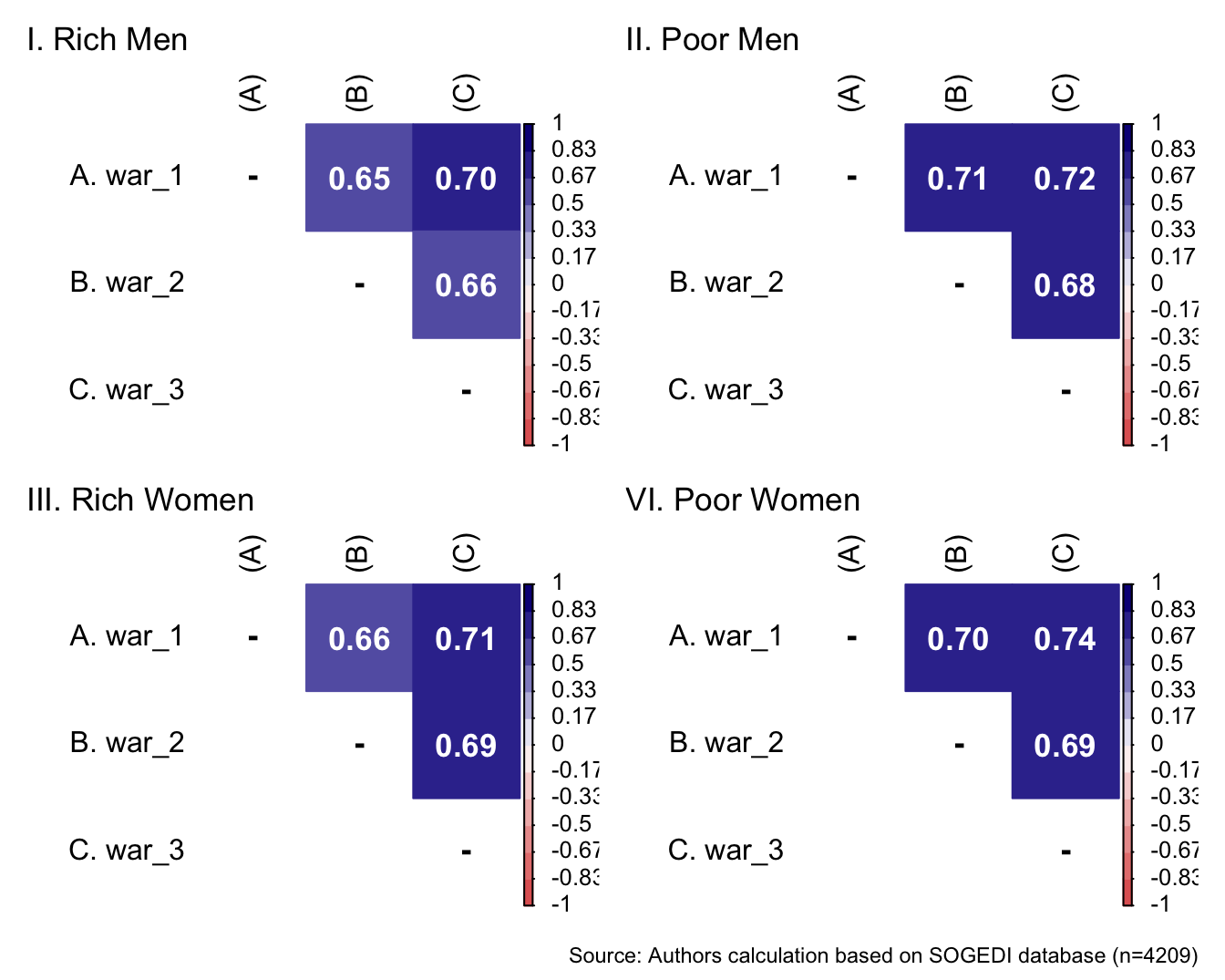
Reliability
mi_variable <- "war"
result2 <- alphas(db_proc, c("war_1", "war_2", "war_3"), mi_variable)

result2$raw_alpha
[1] 0.8808715result2$new_var_summary Min. 1st Qu. Median Mean 3rd Qu. Max.
1.000 3.333 4.000 4.178 5.000 7.000 Confirmatory factor analysis
Mardia’s test for evaluate multivariate normality for each target.
mardia(db_rm[,c("war_1", "war_2", "war_3")],
       na.rm = T, plot=T)
Call: mardia(x = db_rm[, c(“war_1”, “war_2”, “war_3”)], na.rm = T, plot = T)
Mardia tests of multivariate skew and kurtosis Use describe(x) the to get univariate tests n.obs = 1043 num.vars = 3 b1p = 0.34 skew = 59.18 with probability <= 0.0000000052 small sample skew = 59.43 with probability <= 0.0000000046 b2p = 20.73 kurtosis = 16.9 with probability <= 0
mardia(db_pm[,c("war_1", "war_2", "war_3")],
       na.rm = T, plot=T)
Call: mardia(x = db_pm[, c(“war_1”, “war_2”, “war_3”)], na.rm = T, plot = T)
Mardia tests of multivariate skew and kurtosis Use describe(x) the to get univariate tests n.obs = 1058 num.vars = 3 b1p = 0.51 skew = 89.74 with probability <= 0.000000000000006 small sample skew = 90.12 with probability <= 0.0000000000000051 b2p = 27.61 kurtosis = 37.43 with probability <= 0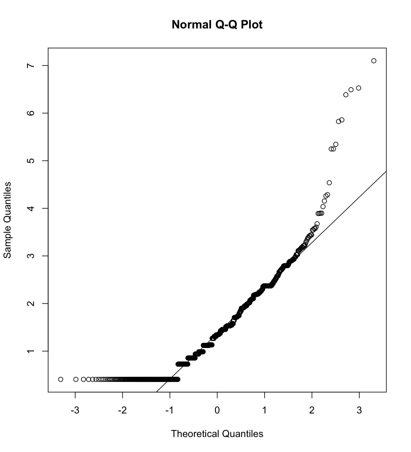
mardia(db_rw[,c("war_1", "war_2", "war_3")],
       na.rm = T, plot=T)
Call: mardia(x = db_rw[, c(“war_1”, “war_2”, “war_3”)], na.rm = T, plot = T)
Mardia tests of multivariate skew and kurtosis Use describe(x) the to get univariate tests n.obs = 1056 num.vars = 3 b1p = 0.25 skew = 44.72 with probability <= 0.0000024 small sample skew = 44.91 with probability <= 0.0000023 b2p = 22.3 kurtosis = 21.67 with probability <= 0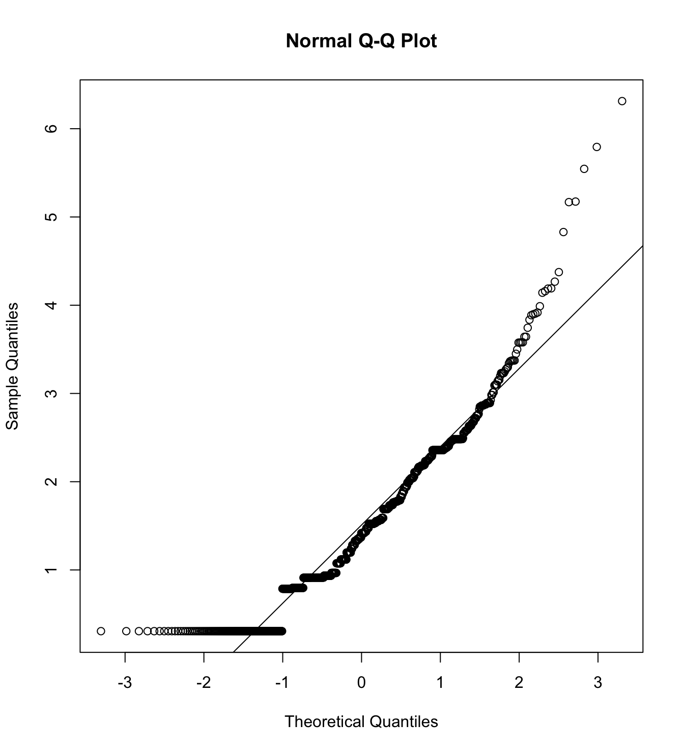
mardia(db_pw[,c("war_1", "war_2", "war_3")],
       na.rm = T, plot=T)
Call: mardia(x = db_pw[, c(“war_1”, “war_2”, “war_3”)], na.rm = T, plot = T)
Mardia tests of multivariate skew and kurtosis Use describe(x) the to get univariate tests n.obs = 1052 num.vars = 3 b1p = 1.6 skew = 279.82 with probability <= 0.0000000000000000000000000000000000000000000000000000028 small sample skew = 281.02 with probability <= 0.0000000000000000000000000000000000000000000000000000016 b2p = 26.18 kurtosis = 33.09 with probability <= 0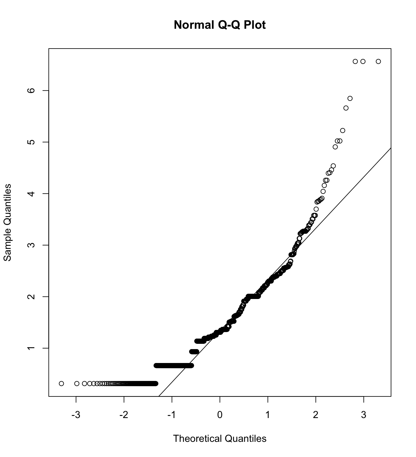
We first specify the factorial structure of the items, then fit models using a robust maximum likelihood estimator for the entire sample as well as for each country individually. The goodnes of fit indicators are shown.
# model
model_cfa <- '
  warmth =~ war_1 + war_2 + war_3
   '

# estimation
# overall
m10_cfa_rm <- cfa(model = model_cfa,
              data = subset(db_proc, target == "Rich.Men"),
              estimator = "MLR",
              ordered = F,
              std.lv = F)

m10_cfa_pm <- cfa(model = model_cfa,
              data = subset(db_proc, target == "Poor.Men"),
              estimator = "MLR",
              ordered = F,
              std.lv = F)

m10_cfa_rw <- cfa(model = model_cfa,
              data = subset(db_proc, target == "Rich.Women"),
              estimator = "MLR",
              ordered = F,
              std.lv = F)

m10_cfa_pw <- cfa(model = model_cfa,
              data = subset(db_proc, target == "Poor.Women"),
              estimator = "MLR",
              ordered = F,
              std.lv = F)


# argentina
m10_cfa_rm_arg <- cfa(model = model_cfa,
                 data = subset(db_proc, group == "1.Rich.Men"),
                 estimator = "MLR",
                 ordered = F,
                 std.lv = F)

m10_cfa_pm_arg <- cfa(model = model_cfa,
                 data = subset(db_proc, group == "1.Poor.Men"),
                 estimator = "MLR",
                 ordered = F,
                 std.lv = F)

m10_cfa_rw_arg <- cfa(model = model_cfa,
                 data = subset(db_proc, group == "1.Rich.Women"),
                 estimator = "MLR",
                 ordered = F,
                 std.lv = F)

m10_cfa_pw_arg <- cfa(model = model_cfa,
                 data = subset(db_proc, group == "1.Poor.Women"),
                 estimator = "MLR",
                 ordered = F,
                 std.lv = F)

# chile
m10_cfa_rm_cl <- cfa(model = model_cfa,
                     data = subset(db_proc, group == "3.Rich.Men"),
                     estimator = "MLR",
                     ordered = F,
                     std.lv = F)

m10_cfa_pm_cl <- cfa(model = model_cfa,
                     data = subset(db_proc, group == "3.Poor.Men"),
                     estimator = "MLR",
                     ordered = F,
                     std.lv = F)

m10_cfa_rw_cl <- cfa(model = model_cfa,
                     data = subset(db_proc, group == "3.Rich.Women"),
                     estimator = "MLR",
                     ordered = F,
                     std.lv = F)

m10_cfa_pw_cl <- cfa(model = model_cfa,
                     data = subset(db_proc, group == "3.Poor.Women"),
                     estimator = "MLR",
                     ordered = F,
                     std.lv = F)

# colombia
m10_cfa_rm_col <- cfa(model = model_cfa,
                     data = subset(db_proc, group == "4.Rich.Men"),
                     estimator = "MLR",
                     ordered = F,
                     std.lv = F)

m10_cfa_pm_col <- cfa(model = model_cfa,
                     data = subset(db_proc, group == "4.Poor.Men"),
                     estimator = "MLR",
                     ordered = F,
                     std.lv = F)

m10_cfa_rw_col <- cfa(model = model_cfa,
                     data = subset(db_proc, group == "4.Rich.Women"),
                     estimator = "MLR",
                     ordered = F,
                     std.lv = F)

m10_cfa_pw_col <- cfa(model = model_cfa,
                     data = subset(db_proc, group == "4.Poor.Women"),
                     estimator = "MLR",
                     ordered = F,
                     std.lv = F)

# españa
m10_cfa_rm_esp <- cfa(model = model_cfa,
                     data = subset(db_proc, group == "9.Rich.Men"),
                     estimator = "MLR",
                     ordered = F,
                     std.lv = F)

m10_cfa_pm_esp <- cfa(model = model_cfa,
                     data = subset(db_proc, group == "9.Poor.Men"),
                     estimator = "MLR",
                     ordered = F,
                     std.lv = F)

m10_cfa_rw_esp <- cfa(model = model_cfa,
                     data = subset(db_proc, group == "9.Rich.Women"),
                     estimator = "MLR",
                     ordered = F,
                     std.lv = F)

m10_cfa_pw_esp <- cfa(model = model_cfa,
                     data = subset(db_proc, group == "9.Poor.Women"),
                     estimator = "MLR",
                     ordered = F,
                     std.lv = F)

# mexico
m10_cfa_rm_mex <- cfa(model = model_cfa,
                     data = subset(db_proc, group == "13.Rich.Men"),
                     estimator = "MLR",
                     ordered = F,
                     std.lv = F)

m10_cfa_pm_mex <- cfa(model = model_cfa,
                     data = subset(db_proc, group == "13.Poor.Men"),
                     estimator = "MLR",
                     ordered = F,
                     std.lv = F)

m10_cfa_rw_mex <- cfa(model = model_cfa,
                     data = subset(db_proc, group == "13.Rich.Women"),
                     estimator = "MLR",
                     ordered = F,
                     std.lv = F)

m10_cfa_pw_mex <- cfa(model = model_cfa,
                     data = subset(db_proc, group == "13.Poor.Women"),
                     estimator = "MLR",
                     ordered = F,
                     std.lv = F)
colnames_fit <- c("","Target","$N$","Estimator","$\\chi^2$ (df)","CFI","TLI","RMSEA 90% CI [Lower-Upper]", "SRMR", "AIC")
bind_rows(
cfa_tab_fit(
models = list(m10_cfa_rm, m10_cfa_rm_arg, m10_cfa_rm_cl, m10_cfa_rm_col, m10_cfa_rm_esp, m10_cfa_rm_mex),
country_names = c("Overall scores", "Argentina", "Chile", "Colombia", "Spain", "México")
)$sum_fit %>%
mutate(target = "Rich Men")
,
cfa_tab_fit(
models = list(m10_cfa_pm, m10_cfa_pm_arg, m10_cfa_pm_cl, m10_cfa_pm_col, m10_cfa_pm_esp, m10_cfa_pm_mex),
country_names = c("Overall scores", "Argentina", "Chile", "Colombia", "Spain", "México")
)$sum_fit %>%
mutate(target = "Poor Men")
,
cfa_tab_fit(
models = list(m10_cfa_rw, m10_cfa_rw_arg, m10_cfa_rw_cl, m10_cfa_rw_col, m10_cfa_rw_esp, m10_cfa_rw_mex),
country_names = c("Overall scores", "Argentina", "Chile", "Colombia", "Spain", "México")
)$sum_fit %>%
mutate(target = "Rich Women")
,
cfa_tab_fit(
models = list(m10_cfa_pw, m10_cfa_pw_arg, m10_cfa_pw_cl, m10_cfa_pw_col, m10_cfa_pw_esp, m10_cfa_pw_mex),
country_names = c("Overall scores", "Argentina", "Chile", "Colombia", "Spain", "México")
)$sum_fit %>%
mutate(target = "Poor Women")
) %>%
select(country, target, everything()) %>%
mutate(country = factor(country, levels = c("Overall scores", "Argentina", "Chile", "Colombia", "Spain", "México"))) %>%
group_by(country) %>%
arrange(country) %>%
mutate(country = if_else(duplicated(country), NA, country)) %>%
kableExtra::kable(
format = "markdown",
digits = 3,
booktabs = TRUE,
col.names = colnames_fit,
caption = NULL
) %>%
kableExtra::kable_styling(
full_width = TRUE,
font_size = 11,
latex_options = "HOLD_position",
bootstrap_options = c("striped", "bordered")
) %>%
kableExtra::collapse_rows(columns = 1)| Target | \(N\) | Estimator | \(\chi^2\) (df) | CFI | TLI | RMSEA 90% CI [Lower-Upper] | SRMR | AIC | |
|---|---|---|---|---|---|---|---|---|---|
| Overall scores | Rich Men | 1043 | ML | 0 (0) | 1 | 1 | 0 [0-0] | 0 | 9332.975 |
| Poor Men | 1058 | ML | 0 (0) | 1 | 1 | 0 [0-0] | 0 | 9057.274 | |
| Rich Women | 1056 | ML | 0 (0) | 1 | 1 | 0 [0-0] | 0 | 9612.983 | |
| Poor Women | 1052 | ML | 0 (0) | 1 | 1 | 0 [0-0] | 0 | 8793.574 | |
| Argentina | Rich Men | 216 | ML | 0 (0) | 1 | 1 | 0 [0-0] | 0 | 1934.807 |
| Poor Men | 219 | ML | 0 (0) | 1 | 1 | 0 [0-0] | 0 | 1911.227 | |
| Rich Women | 207 | ML | 0 (0) | 1 | 1 | 0 [0-0] | 0 | 1837.963 | |
| Poor Women | 215 | ML | 0 (0) | 1 | 1 | 0 [0-0] | 0 | 1740.027 | |
| Chile | Rich Men | 217 | ML | 0 (0) | 1 | 1 | 0 [0-0] | 0 | 1990.219 |
| Poor Men | 215 | ML | 0 (0) | 1 | 1 | 0 [0-0] | 0 | 1893.533 | |
| Rich Women | 223 | ML | 0 (0) | 1 | 1 | 0 [0-0] | 0 | 2044.606 | |
| Poor Women | 205 | ML | 0 (0) | 1 | 1 | 0 [0-0] | 0 | 1781.331 | |
| Colombia | Rich Men | 206 | ML | 0 (0) | 1 | 1 | 0 [0-0] | 0 | 1841.377 |
| Poor Men | 214 | ML | 0 (0) | 1 | 1 | 0 [0-0] | 0 | 1820.878 | |
| Rich Women | 199 | ML | 0 (0) | 1 | 1 | 0 [0-0] | 0 | 1866.105 | |
| Poor Women | 205 | ML | 0 (0) | 1 | 1 | 0 [0-0] | 0 | 1798.193 | |
| Spain | Rich Men | 195 | ML | 0 (0) | 1 | 1 | 0 [0-0] | 0 | 1604.356 |
| Poor Men | 213 | ML | 0 (0) | 1 | 1 | 0 [0-0] | 0 | 1558.266 | |
| Rich Women | 212 | ML | 0 (0) | 1 | 1 | 0 [0-0] | 0 | 1722.409 | |
| Poor Women | 211 | ML | 0 (0) | 1 | 1 | 0 [0-0] | 0 | 1619.085 | |
| México | Rich Men | 209 | ML | 0 (0) | 1 | 1 | 0 [0-0] | 0 | 1931.478 |
| Poor Men | 197 | ML | 0 (0) | 1 | 1 | 0 [0-0] | 0 | 1784.471 | |
| Rich Women | 215 | ML | 0 (0) | 1 | 1 | 0 [0-0] | 0 | 2069.670 | |
| Poor Women | 216 | ML | 0 (0) | 1 | 1 | 0 [0-0] | 0 | 1773.125 |
5.4.4 Competence
We included the immorality scale in an exploratory manner. The items are form the published article from Sánchez-Castelló et al. (2022).
Descriptive analysis
bind_rows(
psych::describe(db_rm[,c("com_1", "com_2", "com_3")]) %>%
    as_tibble() %>%
    mutate(target = "Rich Men")
,
psych::describe(db_pm[,c("com_1", "com_2", "com_3")]) %>%
    as_tibble() %>%
    mutate(target = "Poor Men")
,
psych::describe(db_rw[,c("com_1", "com_2", "com_3")]) %>%
    as_tibble() %>%
    mutate(target = "Rich Women")
,
psych::describe(db_pw[,c("com_1", "com_2", "com_3")]) %>%
    as_tibble() %>%
    mutate(target = "Poor Women")
) %>%
  mutate(vars = paste0("co_", vars)) %>%
  select(target, everything()) %>%
  group_by(target) %>%
  mutate(target = if_else(duplicated(target), NA, target)) %>%
kableExtra::kable(format = "markdown", digits = 3)| target | vars | n | mean | sd | median | trimmed | mad | min | max | range | skew | kurtosis | se |
|---|---|---|---|---|---|---|---|---|---|---|---|---|---|
| Rich Men | co_1 | 1043 | 5.017 | 1.396 | 5 | 5.104 | 1.483 | 1 | 7 | 6 | -0.500 | 0.084 | 0.043 |
| co_2 | 1043 | 5.058 | 1.458 | 5 | 5.175 | 1.483 | 1 | 7 | 6 | -0.615 | 0.046 | 0.045 | |
| co_3 | 1043 | 4.825 | 1.418 | 5 | 4.879 | 1.483 | 1 | 7 | 6 | -0.393 | -0.149 | 0.044 | |
| Poor Men | co_1 | 1058 | 4.262 | 1.393 | 4 | 4.268 | 1.483 | 1 | 7 | 6 | 0.007 | -0.126 | 0.043 |
| co_2 | 1058 | 4.573 | 1.418 | 4 | 4.590 | 1.483 | 1 | 7 | 6 | -0.178 | -0.133 | 0.044 | |
| co_3 | 1058 | 4.232 | 1.420 | 4 | 4.231 | 1.483 | 1 | 7 | 6 | 0.033 | -0.112 | 0.044 | |
| Rich Women | co_1 | 1056 | 4.863 | 1.420 | 5 | 4.937 | 1.483 | 1 | 7 | 6 | -0.482 | 0.034 | 0.044 |
| co_2 | 1056 | 4.808 | 1.469 | 5 | 4.891 | 1.483 | 1 | 7 | 6 | -0.496 | -0.042 | 0.045 | |
| co_3 | 1056 | 4.680 | 1.514 | 5 | 4.764 | 1.483 | 1 | 7 | 6 | -0.476 | -0.068 | 0.047 | |
| Poor Women | co_1 | 1052 | 4.643 | 1.437 | 4 | 4.648 | 1.483 | 1 | 7 | 6 | -0.011 | -0.523 | 0.044 |
| co_2 | 1052 | 4.900 | 1.399 | 5 | 4.943 | 1.483 | 1 | 7 | 6 | -0.181 | -0.418 | 0.043 | |
| co_3 | 1052 | 4.630 | 1.430 | 4 | 4.643 | 1.483 | 1 | 7 | 6 | -0.085 | -0.301 | 0.044 |
p1 <- wrap_elements(
    ~corrplot::corrplot(
      fit_correlations(db_rm, c("com_1", "com_2", "com_3")),
      method = "color",
      type = "upper",
      col = colorRampPalette(c("#E16462", "white", "#0D0887"))(12),
      tl.pos = "lt",
      tl.col = "black",
      addrect = 2,
      rect.col = "black",
      addCoef.col = "white",
      cl.cex = 0.8,
      cl.align.text = 'l',
      number.cex = 1.1,
      na.label = "-",
      bg = "white"
    )
  ) + labs(title = "I. Rich Men")


p2 <- wrap_elements(
    ~corrplot::corrplot(
      fit_correlations(db_pm, c("com_1", "com_2", "com_3")),
      method = "color",
      type = "upper",
      col = colorRampPalette(c("#E16462", "white", "#0D0887"))(12),
      tl.pos = "lt",
      tl.col = "black",
      addrect = 2,
      rect.col = "black",
      addCoef.col = "white",
      cl.cex = 0.8,
      cl.align.text = 'l',
      number.cex = 1.1,
      na.label = "-",
      bg = "white"
    )
  ) + labs(title = "II. Poor Men")

p3 <- wrap_elements(
    ~corrplot::corrplot(
      fit_correlations(db_rw, c("com_1", "com_2", "com_3")),
      method = "color",
      type = "upper",
      col = colorRampPalette(c("#E16462", "white", "#0D0887"))(12),
      tl.pos = "lt",
      tl.col = "black",
      addrect = 2,
      rect.col = "black",
      addCoef.col = "white",
      cl.cex = 0.8,
      cl.align.text = 'l',
      number.cex = 1.1,
      na.label = "-",
      bg = "white"
    )
  ) + labs(title = "III. Rich Women")

p4 <- wrap_elements(
    ~corrplot::corrplot(
      fit_correlations(db_pw, c("com_1", "com_2", "com_3")),
      method = "color",
      type = "upper",
      col = colorRampPalette(c("#E16462", "white", "#0D0887"))(12),
      tl.pos = "lt",
      tl.col = "black",
      addrect = 2,
      rect.col = "black",
      addCoef.col = "white",
      cl.cex = 0.8,
      cl.align.text = 'l',
      number.cex = 1.1,
      na.label = "-",
      bg = "white"
    )
  )+ labs(title = "VI. Poor Women")

a <- p1 + p2

b <- p3 + p4

a/b +
    plot_annotation(
      caption = paste0(
        "Source: Authors calculation based on SOGEDI",
        " database (n=", nrow(db_proc), ")"
      )
    )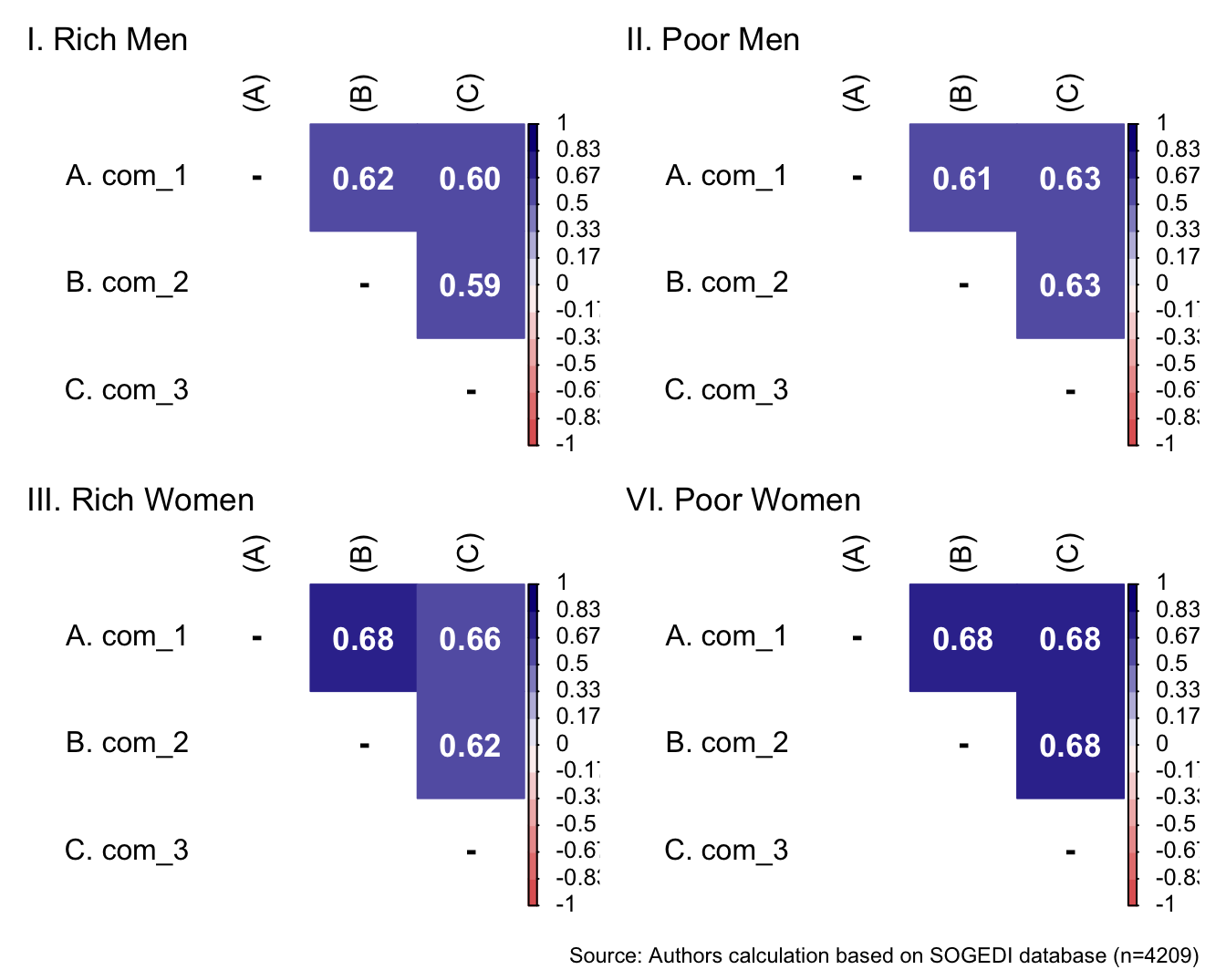
Reliability
mi_variable <- "com"
result2 <- alphas(db_proc, c("com_1", "com_2", "com_3"), mi_variable)

result2$raw_alpha
[1] 0.8456987result2$new_var_summary Min. 1st Qu. Median Mean 3rd Qu. Max.
1.000 4.000 4.667 4.707 5.667 7.000 Confirmatory factor analysis
Mardia’s test for evaluate multivariate normality for each target.
mardia(db_rm[,c("com_1", "com_2", "com_3")],
       na.rm = T, plot=T)
Call: mardia(x = db_rm[, c(“com_1”, “com_2”, “com_3”)], na.rm = T, plot = T)
Mardia tests of multivariate skew and kurtosis Use describe(x) the to get univariate tests n.obs = 1043 num.vars = 3 b1p = 1.53 skew = 265.7 with probability <= 0.0000000000000000000000000000000000000000000000000027 small sample skew = 266.85 with probability <= 0.0000000000000000000000000000000000000000000000000015 b2p = 24.08 kurtosis = 26.77 with probability <= 0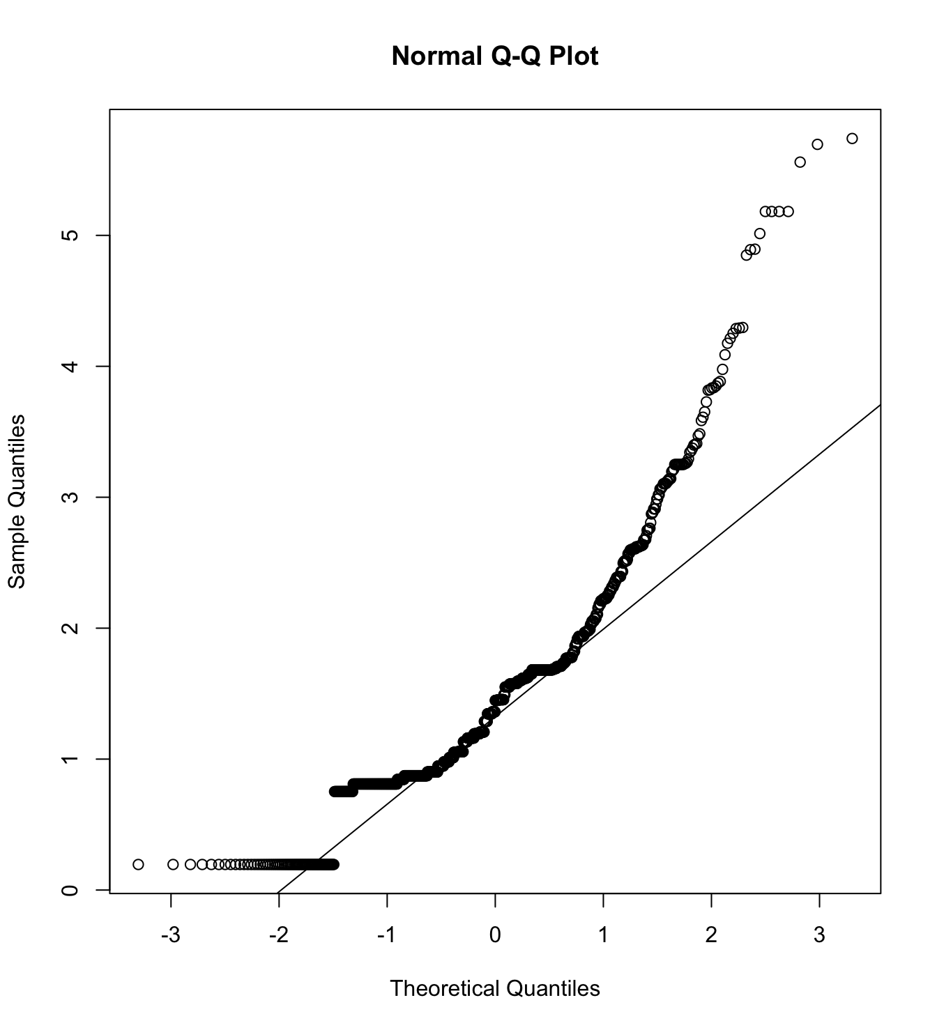
mardia(db_pm[,c("com_1", "com_2", "com_3")],
       na.rm = T, plot=T)
Call: mardia(x = db_pm[, c(“com_1”, “com_2”, “com_3”)], na.rm = T, plot = T)
Mardia tests of multivariate skew and kurtosis Use describe(x) the to get univariate tests n.obs = 1058 num.vars = 3 b1p = 1.14 skew = 200.6 with probability <= 0.00000000000000000000000000000000000012 small sample skew = 201.46 with probability <= 0.00000000000000000000000000000000000008 b2p = 23.72 kurtosis = 25.89 with probability <= 0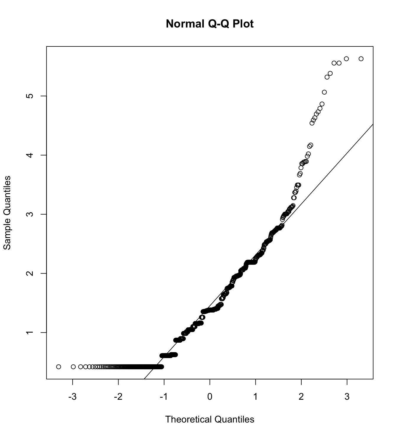
mardia(db_rw[,c("com_1", "com_2", "com_3")],
       na.rm = T, plot=T)
Call: mardia(x = db_rw[, c(“com_1”, “com_2”, “com_3”)], na.rm = T, plot = T)
Mardia tests of multivariate skew and kurtosis Use describe(x) the to get univariate tests n.obs = 1056 num.vars = 3 b1p = 1.64 skew = 288.46 with probability <= 0.000000000000000000000000000000000000000000000000000000043 small sample skew = 289.69 with probability <= 0.000000000000000000000000000000000000000000000000000000023 b2p = 25.42 kurtosis = 30.91 with probability <= 0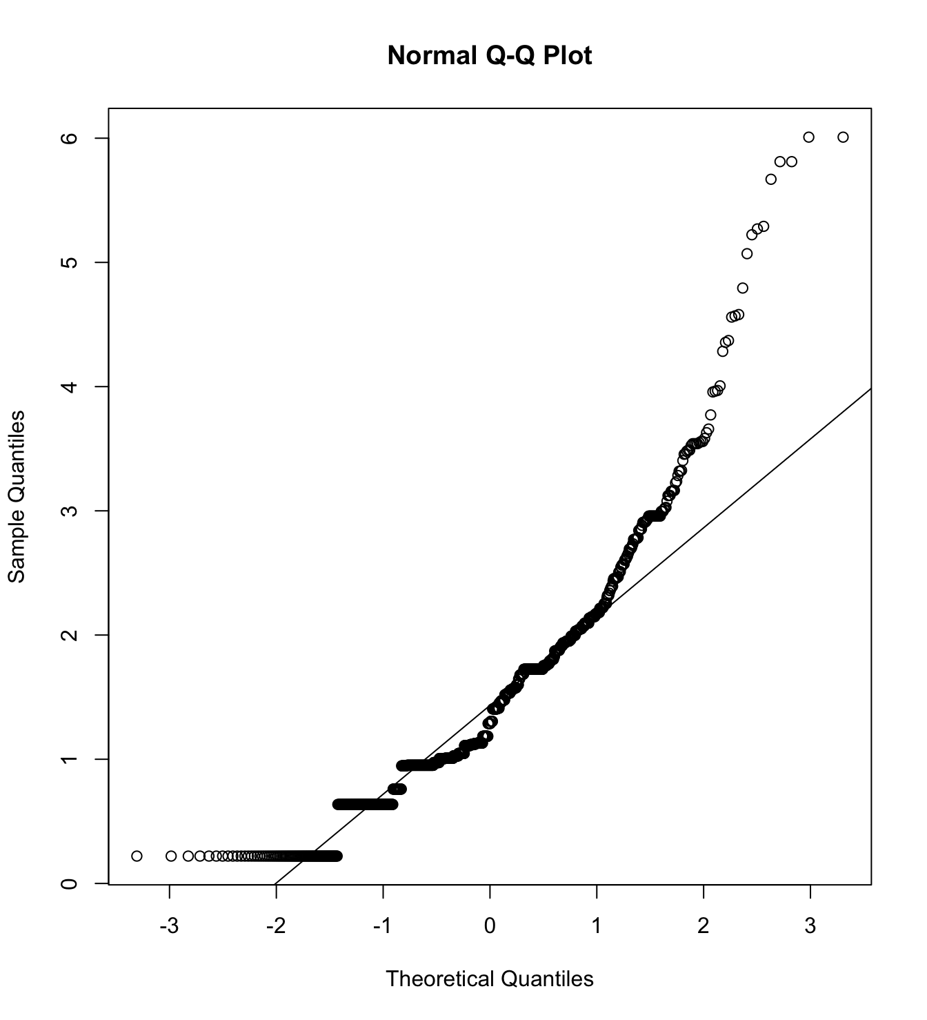
mardia(db_pw[,c("com_1", "com_2", "com_3")],
       na.rm = T, plot=T)
Call: mardia(x = db_pw[, c(“com_1”, “com_2”, “com_3”)], na.rm = T, plot = T)
Mardia tests of multivariate skew and kurtosis Use describe(x) the to get univariate tests n.obs = 1052 num.vars = 3 b1p = 0.99 skew = 173.94 with probability <= 0.000000000000000000000000000000042 small sample skew = 174.68 with probability <= 0.00000000000000000000000000000003 b2p = 20.86 kurtosis = 17.36 with probability <= 0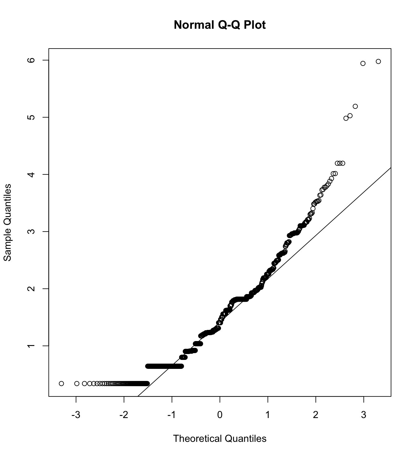
We first specify the factorial structure of the items, then fit models using a robust maximum likelihood estimator for the entire sample as well as for each country individually. The goodnes of fit indicators are shown.
# model
model_cfa <- '
  competence =~ com_1 + com_2 + com_3
   '

# estimation
# overall
m11_cfa_rm <- cfa(model = model_cfa,
              data = subset(db_proc, target == "Rich.Men"),
              estimator = "MLR",
              ordered = F,
              std.lv = F)

m11_cfa_pm <- cfa(model = model_cfa,
              data = subset(db_proc, target == "Poor.Men"),
              estimator = "MLR",
              ordered = F,
              std.lv = F)

m11_cfa_rw <- cfa(model = model_cfa,
              data = subset(db_proc, target == "Rich.Women"),
              estimator = "MLR",
              ordered = F,
              std.lv = F)

m11_cfa_pw <- cfa(model = model_cfa,
              data = subset(db_proc, target == "Poor.Women"),
              estimator = "MLR",
              ordered = F,
              std.lv = F)


# argentina
m11_cfa_rm_arg <- cfa(model = model_cfa,
                 data = subset(db_proc, group == "1.Rich.Men"),
                 estimator = "MLR",
                 ordered = F,
                 std.lv = F)

m11_cfa_pm_arg <- cfa(model = model_cfa,
                 data = subset(db_proc, group == "1.Poor.Men"),
                 estimator = "MLR",
                 ordered = F,
                 std.lv = F)

m11_cfa_rw_arg <- cfa(model = model_cfa,
                 data = subset(db_proc, group == "1.Rich.Women"),
                 estimator = "MLR",
                 ordered = F,
                 std.lv = F)

m11_cfa_pw_arg <- cfa(model = model_cfa,
                 data = subset(db_proc, group == "1.Poor.Women"),
                 estimator = "MLR",
                 ordered = F,
                 std.lv = F)

# chile
m11_cfa_rm_cl <- cfa(model = model_cfa,
                     data = subset(db_proc, group == "3.Rich.Men"),
                     estimator = "MLR",
                     ordered = F,
                     std.lv = F)

m11_cfa_pm_cl <- cfa(model = model_cfa,
                     data = subset(db_proc, group == "3.Poor.Men"),
                     estimator = "MLR",
                     ordered = F,
                     std.lv = F)

m11_cfa_rw_cl <- cfa(model = model_cfa,
                     data = subset(db_proc, group == "3.Rich.Women"),
                     estimator = "MLR",
                     ordered = F,
                     std.lv = F)

m11_cfa_pw_cl <- cfa(model = model_cfa,
                     data = subset(db_proc, group == "3.Poor.Women"),
                     estimator = "MLR",
                     ordered = F,
                     std.lv = F)

# colombia
m11_cfa_rm_col <- cfa(model = model_cfa,
                     data = subset(db_proc, group == "4.Rich.Men"),
                     estimator = "MLR",
                     ordered = F,
                     std.lv = F)

m11_cfa_pm_col <- cfa(model = model_cfa,
                     data = subset(db_proc, group == "4.Poor.Men"),
                     estimator = "MLR",
                     ordered = F,
                     std.lv = F)

m11_cfa_rw_col <- cfa(model = model_cfa,
                     data = subset(db_proc, group == "4.Rich.Women"),
                     estimator = "MLR",
                     ordered = F,
                     std.lv = F)

m11_cfa_pw_col <- cfa(model = model_cfa,
                     data = subset(db_proc, group == "4.Poor.Women"),
                     estimator = "MLR",
                     ordered = F,
                     std.lv = F)

# españa
m11_cfa_rm_esp <- cfa(model = model_cfa,
                     data = subset(db_proc, group == "9.Rich.Men"),
                     estimator = "MLR",
                     ordered = F,
                     std.lv = F)

m11_cfa_pm_esp <- cfa(model = model_cfa,
                     data = subset(db_proc, group == "9.Poor.Men"),
                     estimator = "MLR",
                     ordered = F,
                     std.lv = F)

m11_cfa_rw_esp <- cfa(model = model_cfa,
                     data = subset(db_proc, group == "9.Rich.Women"),
                     estimator = "MLR",
                     ordered = F,
                     std.lv = F)

m11_cfa_pw_esp <- cfa(model = model_cfa,
                     data = subset(db_proc, group == "9.Poor.Women"),
                     estimator = "MLR",
                     ordered = F,
                     std.lv = F)

# mexico
m11_cfa_rm_mex <- cfa(model = model_cfa,
                     data = subset(db_proc, group == "13.Rich.Men"),
                     estimator = "MLR",
                     ordered = F,
                     std.lv = F)

m11_cfa_pm_mex <- cfa(model = model_cfa,
                     data = subset(db_proc, group == "13.Poor.Men"),
                     estimator = "MLR",
                     ordered = F,
                     std.lv = F)

m11_cfa_rw_mex <- cfa(model = model_cfa,
                     data = subset(db_proc, group == "13.Rich.Women"),
                     estimator = "MLR",
                     ordered = F,
                     std.lv = F)

m11_cfa_pw_mex <- cfa(model = model_cfa,
                     data = subset(db_proc, group == "13.Poor.Women"),
                     estimator = "MLR",
                     ordered = F,
                     std.lv = F)
colnames_fit <- c("","Target","$N$","Estimator","$\\chi^2$ (df)","CFI","TLI","RMSEA 90% CI [Lower-Upper]", "SRMR", "AIC")
bind_rows(
cfa_tab_fit(
models = list(m11_cfa_rm, m11_cfa_rm_arg, m11_cfa_rm_cl, m11_cfa_rm_col, m11_cfa_rm_esp, m11_cfa_rm_mex),
country_names = c("Overall scores", "Argentina", "Chile", "Colombia", "Spain", "México")
)$sum_fit %>%
mutate(target = "Rich Men")
,
cfa_tab_fit(
models = list(m11_cfa_pm, m11_cfa_pm_arg, m11_cfa_pm_cl, m11_cfa_pm_col, m11_cfa_pm_esp, m11_cfa_pm_mex),
country_names = c("Overall scores", "Argentina", "Chile", "Colombia", "Spain", "México")
)$sum_fit %>%
mutate(target = "Poor Men")
,
cfa_tab_fit(
models = list(m11_cfa_rw, m11_cfa_rw_arg, m11_cfa_rw_cl, m11_cfa_rw_col, m11_cfa_rw_esp, m11_cfa_rw_mex),
country_names = c("Overall scores", "Argentina", "Chile", "Colombia", "Spain", "México")
)$sum_fit %>%
mutate(target = "Rich Women")
,
cfa_tab_fit(
models = list(m11_cfa_pw, m11_cfa_pw_arg, m11_cfa_pw_cl, m11_cfa_pw_col, m11_cfa_pw_esp, m11_cfa_pw_mex),
country_names = c("Overall scores", "Argentina", "Chile", "Colombia", "Spain", "México")
)$sum_fit %>%
mutate(target = "Poor Women")
) %>%
select(country, target, everything()) %>%
mutate(country = factor(country, levels = c("Overall scores", "Argentina", "Chile", "Colombia", "Spain", "México"))) %>%
group_by(country) %>%
arrange(country) %>%
mutate(country = if_else(duplicated(country), NA, country)) %>%
kableExtra::kable(
format = "markdown",
digits = 3,
booktabs = TRUE,
col.names = colnames_fit,
caption = NULL
) %>%
kableExtra::kable_styling(
full_width = TRUE,
font_size = 11,
latex_options = "HOLD_position",
bootstrap_options = c("striped", "bordered")
) %>%
kableExtra::collapse_rows(columns = 1)| Target | \(N\) | Estimator | \(\chi^2\) (df) | CFI | TLI | RMSEA 90% CI [Lower-Upper] | SRMR | AIC | |
|---|---|---|---|---|---|---|---|---|---|
| Overall scores | Rich Men | 1043 | ML | 0 (0) | 1 | 1 | 0 [0-0] | 0 | 9988.796 |
| Poor Men | 1058 | ML | 0 (0) | 1 | 1 | 0 [0-0] | 0 | 9988.798 | |
| Rich Women | 1056 | ML | 0 (0) | 1 | 1 | 0 [0-0] | 0 | 10070.509 | |
| Poor Women | 1052 | ML | 0 (0) | 1 | 1 | 0 [0-0] | 0 | 9690.783 | |
| Argentina | Rich Men | 216 | ML | 0 (0) | 1 | 1 | 0 [0-0] | 0 | 2142.351 |
| Poor Men | 219 | ML | 0 (0) | 1 | 1 | 0 [0-0] | 0 | 2107.183 | |
| Rich Women | 207 | ML | 0 (0) | 1 | 1 | 0 [0-0] | 0 | 1987.870 | |
| Poor Women | 215 | ML | 0 (0) | 1 | 1 | 0 [0-0] | 0 | 2005.088 | |
| Chile | Rich Men | 217 | ML | 0 (0) | 1 | 1 | 0 [0-0] | 0 | 2097.180 |
| Poor Men | 215 | ML | 0 (0) | 1 | 1 | 0 [0-0] | 0 | 2047.067 | |
| Rich Women | 223 | ML | 0 (0) | 1 | 1 | 0 [0-0] | 0 | 2188.017 | |
| Poor Women | 205 | ML | 0 (0) | 1 | 1 | 0 [0-0] | 0 | 1843.429 | |
| Colombia | Rich Men | 206 | ML | 0 (0) | 1 | 1 | 0 [0-0] | 0 | 1893.569 |
| Poor Men | 214 | ML | 0 (0) | 1 | 1 | 0 [0-0] | 0 | 2024.499 | |
| Rich Women | 199 | ML | 0 (0) | 1 | 1 | 0 [0-0] | 0 | 1803.823 | |
| Poor Women | 205 | ML | 0 (0) | 1 | 1 | 0 [0-0] | 0 | 1967.218 | |
| Spain | Rich Men | 195 | ML | 0 (0) | 1 | 1 | 0 [0-0] | 0 | 1698.793 |
| Poor Men | 213 | ML | 0 (0) | 1 | 1 | 0 [0-0] | 0 | 1798.758 | |
| Rich Women | 212 | ML | 0 (0) | 1 | 1 | 0 [0-0] | 0 | 1831.850 | |
| Poor Women | 211 | ML | 0 (0) | 1 | 1 | 0 [0-0] | 0 | 1767.824 | |
| México | Rich Men | 209 | ML | 0 (0) | 1 | 1 | 0 [0-0] | 0 | 2077.541 |
| Poor Men | 197 | ML | 0 (0) | 1 | 1 | 0 [0-0] | 0 | 1907.408 | |
| Rich Women | 215 | ML | 0 (0) | 1 | 1 | 0 [0-0] | 0 | 2199.605 | |
| Poor Women | 216 | ML | 0 (0) | 1 | 1 | 0 [0-0] | 0 | 2024.340 |
5.4.5 Intergroup behavioural tendencies: passive harm
This behavior scale is a combination of two scales by López-Rodríguez et al. (2017) and López-Rodríguez et al. (2016), modified to better fit our context. We utilized the scale from the second paper and made adjustments to some collaboration items to better align it with our objectives and the groups being assessed.
Descriptive analysis
bind_rows(
psych::describe(db_rm[,c("ph_1", "ph_2")]) %>%
    as_tibble() %>%
    mutate(target = "Rich Men")
,
psych::describe(db_pm[,c("ph_1", "ph_2")]) %>%
    as_tibble() %>%
    mutate(target = "Poor Men")
,
psych::describe(db_rw[,c("ph_1", "ph_2")]) %>%
    as_tibble() %>%
    mutate(target = "Rich Women")
,
psych::describe(db_pw[,c("ph_1", "ph_2")]) %>%
    as_tibble() %>%
    mutate(target = "Poor Women")
) %>%
  mutate(vars = paste0("ph_", vars)) %>%
  select(target, everything()) %>%
  group_by(target) %>%
  mutate(target = if_else(duplicated(target), NA, target)) %>%
kableExtra::kable(format = "markdown", digits = 3)| target | vars | n | mean | sd | median | trimmed | mad | min | max | range | skew | kurtosis | se |
|---|---|---|---|---|---|---|---|---|---|---|---|---|---|
| Rich Men | ph_1 | 1043 | 2.424 | 1.637 | 2 | 2.169 | 1.483 | 1 | 7 | 6 | 1.033 | 0.245 | 0.051 |
| ph_2 | 1043 | 2.802 | 1.800 | 2 | 2.574 | 1.483 | 1 | 7 | 6 | 0.683 | -0.535 | 0.056 | |
| Poor Men | ph_1 | 1058 | 2.309 | 1.600 | 2 | 2.053 | 1.483 | 1 | 7 | 6 | 1.063 | 0.195 | 0.049 |
| ph_2 | 1058 | 2.332 | 1.537 | 2 | 2.106 | 1.483 | 1 | 7 | 6 | 0.978 | 0.152 | 0.047 | |
| Rich Women | ph_1 | 1056 | 2.302 | 1.645 | 2 | 2.019 | 1.483 | 1 | 7 | 6 | 1.166 | 0.485 | 0.051 |
| ph_2 | 1056 | 2.460 | 1.657 | 2 | 2.219 | 1.483 | 1 | 7 | 6 | 0.921 | -0.092 | 0.051 | |
| Poor Women | ph_1 | 1052 | 1.754 | 1.297 | 1 | 1.468 | 0.000 | 1 | 7 | 6 | 1.852 | 2.908 | 0.040 |
| ph_2 | 1052 | 1.833 | 1.278 | 1 | 1.587 | 0.000 | 1 | 7 | 6 | 1.522 | 1.600 | 0.039 |
p1 <- wrap_elements(
    ~corrplot::corrplot(
      fit_correlations_pairwise(db_rm, c("ph_1", "ph_2")),
      method = "color",
      type = "upper",
      col = colorRampPalette(c("#E16462", "white", "#0D0887"))(12),
      tl.pos = "lt",
      tl.col = "black",
      addrect = 2,
      rect.col = "black",
      addCoef.col = "white",
      cl.cex = 0.8,
      cl.align.text = 'l',
      number.cex = 1.1,
      na.label = "-",
      bg = "white"
    )
  ) + labs(title = "I. Rich Men")


p2 <- wrap_elements(
    ~corrplot::corrplot(
      fit_correlations_pairwise(db_pm, c("ph_1", "ph_2")),
      method = "color",
      type = "upper",
      col = colorRampPalette(c("#E16462", "white", "#0D0887"))(12),
      tl.pos = "lt",
      tl.col = "black",
      addrect = 2,
      rect.col = "black",
      addCoef.col = "white",
      cl.cex = 0.8,
      cl.align.text = 'l',
      number.cex = 1.1,
      na.label = "-",
      bg = "white"
    )
  ) + labs(title = "II. Poor Men")

p3 <- wrap_elements(
    ~corrplot::corrplot(
      fit_correlations_pairwise(db_rw, c("ph_1", "ph_2")),
      method = "color",
      type = "upper",
      col = colorRampPalette(c("#E16462", "white", "#0D0887"))(12),
      tl.pos = "lt",
      tl.col = "black",
      addrect = 2,
      rect.col = "black",
      addCoef.col = "white",
      cl.cex = 0.8,
      cl.align.text = 'l',
      number.cex = 1.1,
      na.label = "-",
      bg = "white"
    )
  ) + labs(title = "III. Rich Women")

p4 <- wrap_elements(
    ~corrplot::corrplot(
      fit_correlations_pairwise(db_pw, c("ph_1", "ph_2")),
      method = "color",
      type = "upper",
      col = colorRampPalette(c("#E16462", "white", "#0D0887"))(12),
      tl.pos = "lt",
      tl.col = "black",
      addrect = 2,
      rect.col = "black",
      addCoef.col = "white",
      cl.cex = 0.8,
      cl.align.text = 'l',
      number.cex = 1.1,
      na.label = "-",
      bg = "white"
    )
  )+ labs(title = "VI. Poor Women")

a <- p1 + p2

b <- p3 + p4

a/b +
    plot_annotation(
      caption = paste0(
        "Source: Authors calculation based on SOGEDI",
        " database (n=", nrow(db_proc), ")"
      )
    )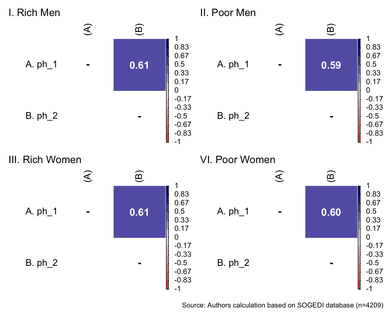
Reliability
5.4.6 Intergroup behavioural tendencies: active harm
This behavior scale is a combination of two scales by Lucía Lopez, modified to better fit our context. We utilized the scale from the second paper and made adjustments to some collaboration items to better align it with our objectives and the groups being assessed.
Descriptive analysis
bind_rows(
psych::describe(db_rm[,c("ah_1", "ah_2")]) %>%
    as_tibble() %>%
    mutate(target = "Rich Men")
,
psych::describe(db_pm[,c("ah_1", "ah_2")]) %>%
    as_tibble() %>%
    mutate(target = "Poor Men")
,
psych::describe(db_rw[,c("ah_1", "ah_2")]) %>%
    as_tibble() %>%
    mutate(target = "Rich Women")
,
psych::describe(db_pw[,c("ah_1", "ah_2")]) %>%
    as_tibble() %>%
    mutate(target = "Poor Women")
) %>%
  mutate(vars = paste0("ah_", vars)) %>%
  select(target, everything()) %>%
  group_by(target) %>%
  mutate(target = if_else(duplicated(target), NA, target)) %>%
kableExtra::kable(format = "markdown", digits = 3)| target | vars | n | mean | sd | median | trimmed | mad | min | max | range | skew | kurtosis | se |
|---|---|---|---|---|---|---|---|---|---|---|---|---|---|
| Rich Men | ah_1 | 1043 | 2.366 | 1.605 | 2 | 2.104 | 1.483 | 1 | 7 | 6 | 1.088 | 0.425 | 0.050 |
| ah_2 | 1043 | 2.256 | 1.600 | 2 | 1.969 | 1.483 | 1 | 7 | 6 | 1.232 | 0.702 | 0.050 | |
| Poor Men | ah_1 | 1058 | 1.725 | 1.277 | 1 | 1.435 | 0.000 | 1 | 7 | 6 | 1.965 | 3.430 | 0.039 |
| ah_2 | 1058 | 1.579 | 1.169 | 1 | 1.277 | 0.000 | 1 | 7 | 6 | 2.339 | 5.361 | 0.036 | |
| Rich Women | ah_1 | 1056 | 2.119 | 1.480 | 1 | 1.868 | 0.000 | 1 | 7 | 6 | 1.272 | 0.901 | 0.046 |
| ah_2 | 1056 | 2.054 | 1.469 | 1 | 1.784 | 0.000 | 1 | 7 | 6 | 1.309 | 0.770 | 0.045 | |
| Poor Women | ah_1 | 1052 | 1.509 | 1.097 | 1 | 1.220 | 0.000 | 1 | 7 | 6 | 2.568 | 6.859 | 0.034 |
| ah_2 | 1052 | 1.432 | 1.003 | 1 | 1.147 | 0.000 | 1 | 6 | 5 | 2.520 | 5.675 | 0.031 |
p1 <- wrap_elements(
    ~corrplot::corrplot(
      fit_correlations_pairwise(db_rm, c("ah_1", "ah_2")),
      method = "color",
      type = "upper",
      col = colorRampPalette(c("#E16462", "white", "#0D0887"))(12),
      tl.pos = "lt",
      tl.col = "black",
      addrect = 2,
      rect.col = "black",
      addCoef.col = "white",
      cl.cex = 0.8,
      cl.align.text = 'l',
      number.cex = 1.1,
      na.label = "-",
      bg = "white"
    )
  ) + labs(title = "I. Rich Men")


p2 <- wrap_elements(
    ~corrplot::corrplot(
      fit_correlations_pairwise(db_pm, c("ah_1", "ah_2")),
      method = "color",
      type = "upper",
      col = colorRampPalette(c("#E16462", "white", "#0D0887"))(12),
      tl.pos = "lt",
      tl.col = "black",
      addrect = 2,
      rect.col = "black",
      addCoef.col = "white",
      cl.cex = 0.8,
      cl.align.text = 'l',
      number.cex = 1.1,
      na.label = "-",
      bg = "white"
    )
  ) + labs(title = "II. Poor Men")

p3 <- wrap_elements(
    ~corrplot::corrplot(
      fit_correlations_pairwise(db_rw, c("ah_1", "ah_2")),
      method = "color",
      type = "upper",
      col = colorRampPalette(c("#E16462", "white", "#0D0887"))(12),
      tl.pos = "lt",
      tl.col = "black",
      addrect = 2,
      rect.col = "black",
      addCoef.col = "white",
      cl.cex = 0.8,
      cl.align.text = 'l',
      number.cex = 1.1,
      na.label = "-",
      bg = "white"
    )
  ) + labs(title = "III. Rich Women")

p4 <- wrap_elements(
    ~corrplot::corrplot(
      fit_correlations_pairwise(db_pw, c("ah_1", "ah_2")),
      method = "color",
      type = "upper",
      col = colorRampPalette(c("#E16462", "white", "#0D0887"))(12),
      tl.pos = "lt",
      tl.col = "black",
      addrect = 2,
      rect.col = "black",
      addCoef.col = "white",
      cl.cex = 0.8,
      cl.align.text = 'l',
      number.cex = 1.1,
      na.label = "-",
      bg = "white"
    )
  )+ labs(title = "VI. Poor Women")

a <- p1 + p2

b <- p3 + p4

a/b +
    plot_annotation(
      caption = paste0(
        "Source: Authors calculation based on SOGEDI",
        " database (n=", nrow(db_proc), ")"
      )
    )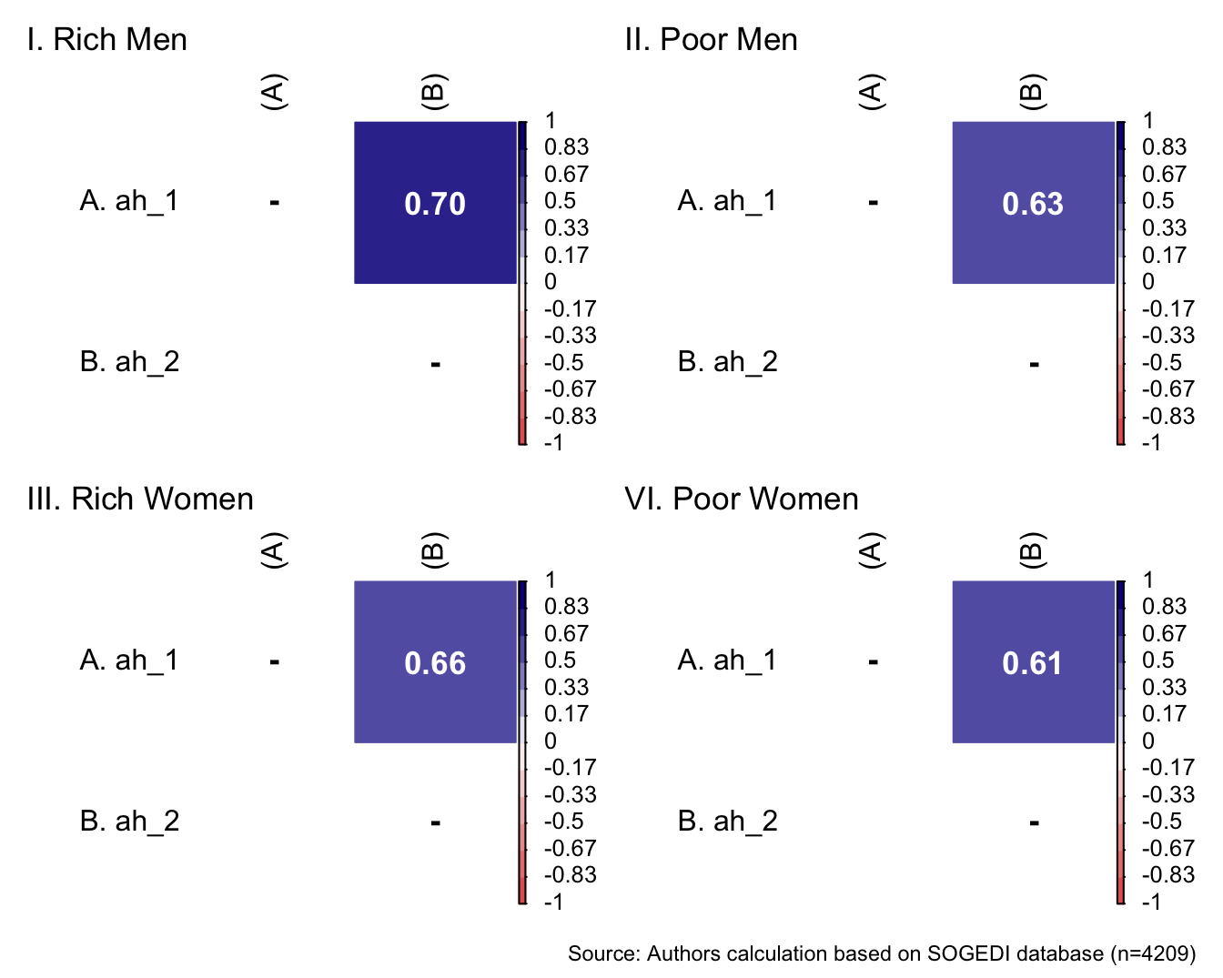
Reliability
5.4.7 Intergroup behavioural tendencies: passive facilitation
This behavior scale is a combination of two scales by Lucía Lopez, modified to better fit our context. We utilized the scale from the second paper and made adjustments to some collaboration items to better align it with our objectives and the groups being assessed.
Descriptive analysis
bind_rows(
psych::describe(db_rm[,c("pf_1", "pf_2")]) %>%
    as_tibble() %>%
    mutate(target = "Rich Men")
,
psych::describe(db_pm[,c("pf_1", "pf_2")]) %>%
    as_tibble() %>%
    mutate(target = "Poor Men")
,
psych::describe(db_rw[,c("pf_1", "pf_2")]) %>%
    as_tibble() %>%
    mutate(target = "Rich Women")
,
psych::describe(db_pw[,c("pf_1", "pf_2")]) %>%
    as_tibble() %>%
    mutate(target = "Poor Women")
) %>%
  mutate(vars = paste0("pf_", vars)) %>%
  select(target, everything()) %>%
  group_by(target) %>%
  mutate(target = if_else(duplicated(target), NA, target)) %>%
kableExtra::kable(format = "markdown", digits = 3)| target | vars | n | mean | sd | median | trimmed | mad | min | max | range | skew | kurtosis | se |
|---|---|---|---|---|---|---|---|---|---|---|---|---|---|
| Rich Men | pf_1 | 1043 | 4.421 | 1.579 | 4 | 4.484 | 1.483 | 1 | 7 | 6 | -0.248 | -0.245 | 0.049 |
| pf_2 | 1043 | 4.417 | 1.775 | 4 | 4.515 | 1.483 | 1 | 7 | 6 | -0.322 | -0.672 | 0.055 | |
| Poor Men | pf_1 | 1058 | 5.112 | 1.653 | 5 | 5.298 | 1.483 | 1 | 7 | 6 | -0.713 | -0.120 | 0.051 |
| pf_2 | 1058 | 3.604 | 1.737 | 4 | 3.534 | 1.483 | 1 | 7 | 6 | 0.204 | -0.694 | 0.053 | |
| Rich Women | pf_1 | 1056 | 4.375 | 1.686 | 4 | 4.435 | 1.483 | 1 | 7 | 6 | -0.216 | -0.568 | 0.052 |
| pf_2 | 1056 | 4.577 | 1.766 | 5 | 4.694 | 1.483 | 1 | 7 | 6 | -0.369 | -0.632 | 0.054 | |
| Poor Women | pf_1 | 1052 | 5.462 | 1.552 | 6 | 5.673 | 1.483 | 1 | 7 | 6 | -0.914 | 0.337 | 0.048 |
| pf_2 | 1052 | 4.185 | 1.741 | 4 | 4.214 | 1.483 | 1 | 7 | 6 | -0.072 | -0.743 | 0.054 |
p1 <- wrap_elements(
    ~corrplot::corrplot(
      fit_correlations_pairwise(db_rm, c("pf_1", "pf_2")),
      method = "color",
      type = "upper",
      col = colorRampPalette(c("#E16462", "white", "#0D0887"))(12),
      tl.pos = "lt",
      tl.col = "black",
      addrect = 2,
      rect.col = "black",
      addCoef.col = "white",
      cl.cex = 0.8,
      cl.align.text = 'l',
      number.cex = 1.1,
      na.label = "-",
      bg = "white"
    )
  ) + labs(title = "I. Rich Men")


p2 <- wrap_elements(
    ~corrplot::corrplot(
      fit_correlations_pairwise(db_pm, c("pf_1", "pf_2")),
      method = "color",
      type = "upper",
      col = colorRampPalette(c("#E16462", "white", "#0D0887"))(12),
      tl.pos = "lt",
      tl.col = "black",
      addrect = 2,
      rect.col = "black",
      addCoef.col = "white",
      cl.cex = 0.8,
      cl.align.text = 'l',
      number.cex = 1.1,
      na.label = "-",
      bg = "white"
    )
  ) + labs(title = "II. Poor Men")

p3 <- wrap_elements(
    ~corrplot::corrplot(
      fit_correlations_pairwise(db_rw, c("pf_1", "pf_2")),
      method = "color",
      type = "upper",
      col = colorRampPalette(c("#E16462", "white", "#0D0887"))(12),
      tl.pos = "lt",
      tl.col = "black",
      addrect = 2,
      rect.col = "black",
      addCoef.col = "white",
      cl.cex = 0.8,
      cl.align.text = 'l',
      number.cex = 1.1,
      na.label = "-",
      bg = "white"
    )
  ) + labs(title = "III. Rich Women")

p4 <- wrap_elements(
    ~corrplot::corrplot(
      fit_correlations_pairwise(db_pw, c("pf_1", "pf_2")),
      method = "color",
      type = "upper",
      col = colorRampPalette(c("#E16462", "white", "#0D0887"))(12),
      tl.pos = "lt",
      tl.col = "black",
      addrect = 2,
      rect.col = "black",
      addCoef.col = "white",
      cl.cex = 0.8,
      cl.align.text = 'l',
      number.cex = 1.1,
      na.label = "-",
      bg = "white"
    )
  )+ labs(title = "VI. Poor Women")

a <- p1 + p2

b <- p3 + p4

a/b +
    plot_annotation(
      caption = paste0(
        "Source: Authors calculation based on SOGEDI",
        " database (n=", nrow(db_proc), ")"
      )
    )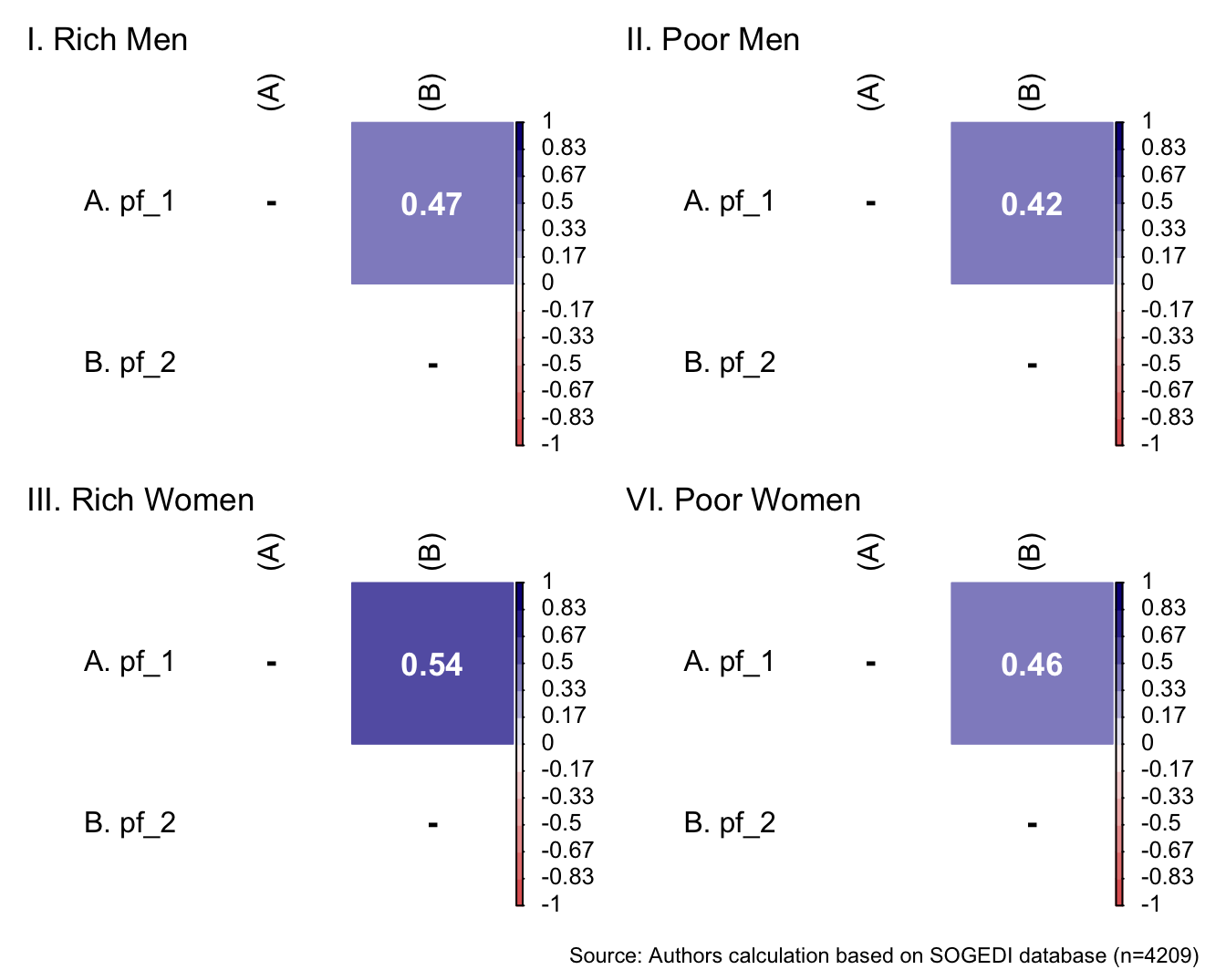
Reliability
5.4.8 Intergroup behavioural tendencies: active facilitation
This behavior scale is a combination of two scales by Lucía Lopez, modified to better fit our context. We utilized the scale from the second paper and made adjustments to some collaboration items to better align it with our objectives and the groups being assessed.
Descriptive analysis
bind_rows(
psych::describe(db_rm[,c("af_1", "af_2")]) %>%
    as_tibble() %>%
    mutate(target = "Rich Men")
,
psych::describe(db_pm[,c("af_1", "af_2")]) %>%
    as_tibble() %>%
    mutate(target = "Poor Men")
,
psych::describe(db_rw[,c("af_1", "af_2")]) %>%
    as_tibble() %>%
    mutate(target = "Rich Women")
,
psych::describe(db_pw[,c("af_1", "af_2")]) %>%
    as_tibble() %>%
    mutate(target = "Poor Women")
) %>%
  mutate(vars = paste0("af_", vars)) %>%
  select(target, everything()) %>%
  group_by(target) %>%
  mutate(target = if_else(duplicated(target), NA, target)) %>%
kableExtra::kable(format = "markdown", digits = 3)| target | vars | n | mean | sd | median | trimmed | mad | min | max | range | skew | kurtosis | se |
|---|---|---|---|---|---|---|---|---|---|---|---|---|---|
| Rich Men | af_1 | 1043 | 3.967 | 1.744 | 4 | 3.964 | 1.483 | 1 | 7 | 6 | -0.069 | -0.718 | 0.054 |
| af_2 | 1043 | 3.975 | 1.710 | 4 | 3.974 | 1.483 | 1 | 7 | 6 | -0.075 | -0.618 | 0.053 | |
| Poor Men | af_1 | 1058 | 3.899 | 1.747 | 4 | 3.876 | 1.483 | 1 | 7 | 6 | 0.075 | -0.813 | 0.054 |
| af_2 | 1058 | 4.541 | 1.632 | 4 | 4.614 | 1.483 | 1 | 7 | 6 | -0.201 | -0.512 | 0.050 | |
| Rich Women | af_1 | 1056 | 4.177 | 1.752 | 4 | 4.209 | 1.483 | 1 | 7 | 6 | -0.089 | -0.771 | 0.054 |
| af_2 | 1056 | 4.200 | 1.754 | 4 | 4.248 | 1.483 | 1 | 7 | 6 | -0.143 | -0.710 | 0.054 | |
| Poor Women | af_1 | 1052 | 4.391 | 1.714 | 4 | 4.441 | 1.483 | 1 | 7 | 6 | -0.115 | -0.731 | 0.053 |
| af_2 | 1052 | 4.935 | 1.558 | 5 | 5.043 | 1.483 | 1 | 7 | 6 | -0.382 | -0.424 | 0.048 |
p1 <- wrap_elements(
    ~corrplot::corrplot(
      fit_correlations_pairwise(db_rm, c("af_1", "af_2")),
      method = "color",
      type = "upper",
      col = colorRampPalette(c("#E16462", "white", "#0D0887"))(12),
      tl.pos = "lt",
      tl.col = "black",
      addrect = 2,
      rect.col = "black",
      addCoef.col = "white",
      cl.cex = 0.8,
      cl.align.text = 'l',
      number.cex = 1.1,
      na.label = "-",
      bg = "white"
    )
  ) + labs(title = "I. Rich Men")


p2 <- wrap_elements(
    ~corrplot::corrplot(
      fit_correlations_pairwise(db_pm, c("af_1", "af_2")),
      method = "color",
      type = "upper",
      col = colorRampPalette(c("#E16462", "white", "#0D0887"))(12),
      tl.pos = "lt",
      tl.col = "black",
      addrect = 2,
      rect.col = "black",
      addCoef.col = "white",
      cl.cex = 0.8,
      cl.align.text = 'l',
      number.cex = 1.1,
      na.label = "-",
      bg = "white"
    )
  ) + labs(title = "II. Poor Men")

p3 <- wrap_elements(
    ~corrplot::corrplot(
      fit_correlations_pairwise(db_rw, c("af_1", "af_2")),
      method = "color",
      type = "upper",
      col = colorRampPalette(c("#E16462", "white", "#0D0887"))(12),
      tl.pos = "lt",
      tl.col = "black",
      addrect = 2,
      rect.col = "black",
      addCoef.col = "white",
      cl.cex = 0.8,
      cl.align.text = 'l',
      number.cex = 1.1,
      na.label = "-",
      bg = "white"
    )
  ) + labs(title = "III. Rich Women")

p4 <- wrap_elements(
    ~corrplot::corrplot(
      fit_correlations_pairwise(db_pw, c("af_1", "af_2")),
      method = "color",
      type = "upper",
      col = colorRampPalette(c("#E16462", "white", "#0D0887"))(12),
      tl.pos = "lt",
      tl.col = "black",
      addrect = 2,
      rect.col = "black",
      addCoef.col = "white",
      cl.cex = 0.8,
      cl.align.text = 'l',
      number.cex = 1.1,
      na.label = "-",
      bg = "white"
    )
  )+ labs(title = "VI. Poor Women")

a <- p1 + p2

b <- p3 + p4

a/b +
    plot_annotation(
      caption = paste0(
        "Source: Authors calculation based on SOGEDI",
        " database (n=", nrow(db_proc), ")"
      )
    )
Reliability
5.4.9 Intergroup affect tendencies: admiration toward
We selected emotions that have been used in various studies that test the BIAS map from Cuddy et al. (2007).
Descriptive analysis
bind_rows(
psych::describe(db_rm[,c("ad_1", "ad_2")]) %>%
    as_tibble() %>%
    mutate(target = "Rich Men")
,
psych::describe(db_pm[,c("ad_1", "ad_2")]) %>%
    as_tibble() %>%
    mutate(target = "Poor Men")
,
psych::describe(db_rw[,c("ad_1", "ad_2")]) %>%
    as_tibble() %>%
    mutate(target = "Rich Women")
,
psych::describe(db_pw[,c("ad_1", "ad_2")]) %>%
    as_tibble() %>%
    mutate(target = "Poor Women")
) %>%
  mutate(vars = paste0("ad_", vars)) %>%
  select(target, everything()) %>%
  group_by(target) %>%
  mutate(target = if_else(duplicated(target), NA, target)) %>%
kableExtra::kable(format = "markdown", digits = 3)| target | vars | n | mean | sd | median | trimmed | mad | min | max | range | skew | kurtosis | se |
|---|---|---|---|---|---|---|---|---|---|---|---|---|---|
| Rich Men | ad_1 | 1043 | 4.046 | 1.812 | 4 | 4.057 | 1.483 | 1 | 7 | 6 | -0.139 | -0.847 | 0.056 |
| ad_2 | 1043 | 4.290 | 1.724 | 4 | 4.351 | 1.483 | 1 | 7 | 6 | -0.213 | -0.638 | 0.053 | |
| Poor Men | ad_1 | 1058 | 3.552 | 1.789 | 4 | 3.473 | 1.483 | 1 | 7 | 6 | 0.145 | -0.804 | 0.055 |
| ad_2 | 1058 | 5.155 | 1.674 | 5 | 5.330 | 1.483 | 1 | 7 | 6 | -0.618 | -0.396 | 0.051 | |
| Rich Women | ad_1 | 1056 | 4.036 | 1.911 | 4 | 4.045 | 2.965 | 1 | 7 | 6 | -0.134 | -1.024 | 0.059 |
| ad_2 | 1056 | 4.619 | 1.747 | 5 | 4.745 | 1.483 | 1 | 7 | 6 | -0.401 | -0.562 | 0.054 | |
| Poor Women | ad_1 | 1052 | 4.288 | 1.821 | 4 | 4.360 | 1.483 | 1 | 7 | 6 | -0.249 | -0.745 | 0.056 |
| ad_2 | 1052 | 5.636 | 1.475 | 6 | 5.831 | 1.483 | 1 | 7 | 6 | -0.989 | 0.514 | 0.045 |
p1 <- wrap_elements(
    ~corrplot::corrplot(
      fit_correlations_pairwise(db_rm, c("ad_1", "ad_2")),
      method = "color",
      type = "upper",
      col = colorRampPalette(c("#E16462", "white", "#0D0887"))(12),
      tl.pos = "lt",
      tl.col = "black",
      addrect = 2,
      rect.col = "black",
      addCoef.col = "white",
      cl.cex = 0.8,
      cl.align.text = 'l',
      number.cex = 1.1,
      na.label = "-",
      bg = "white"
    )
  ) + labs(title = "I. Rich Men")


p2 <- wrap_elements(
    ~corrplot::corrplot(
      fit_correlations_pairwise(db_pm, c("ad_1", "ad_2")),
      method = "color",
      type = "upper",
      col = colorRampPalette(c("#E16462", "white", "#0D0887"))(12),
      tl.pos = "lt",
      tl.col = "black",
      addrect = 2,
      rect.col = "black",
      addCoef.col = "white",
      cl.cex = 0.8,
      cl.align.text = 'l',
      number.cex = 1.1,
      na.label = "-",
      bg = "white"
    )
  ) + labs(title = "II. Poor Men")

p3 <- wrap_elements(
    ~corrplot::corrplot(
      fit_correlations_pairwise(db_rw, c("ad_1", "ad_2")),
      method = "color",
      type = "upper",
      col = colorRampPalette(c("#E16462", "white", "#0D0887"))(12),
      tl.pos = "lt",
      tl.col = "black",
      addrect = 2,
      rect.col = "black",
      addCoef.col = "white",
      cl.cex = 0.8,
      cl.align.text = 'l',
      number.cex = 1.1,
      na.label = "-",
      bg = "white"
    )
  ) + labs(title = "III. Rich Women")

p4 <- wrap_elements(
    ~corrplot::corrplot(
      fit_correlations_pairwise(db_pw, c("ad_1", "ad_2")),
      method = "color",
      type = "upper",
      col = colorRampPalette(c("#E16462", "white", "#0D0887"))(12),
      tl.pos = "lt",
      tl.col = "black",
      addrect = 2,
      rect.col = "black",
      addCoef.col = "white",
      cl.cex = 0.8,
      cl.align.text = 'l',
      number.cex = 1.1,
      na.label = "-",
      bg = "white"
    )
  )+ labs(title = "VI. Poor Women")

a <- p1 + p2

b <- p3 + p4

a/b +
    plot_annotation(
      caption = paste0(
        "Source: Authors calculation based on SOGEDI",
        " database (n=", nrow(db_proc), ")"
      )
    )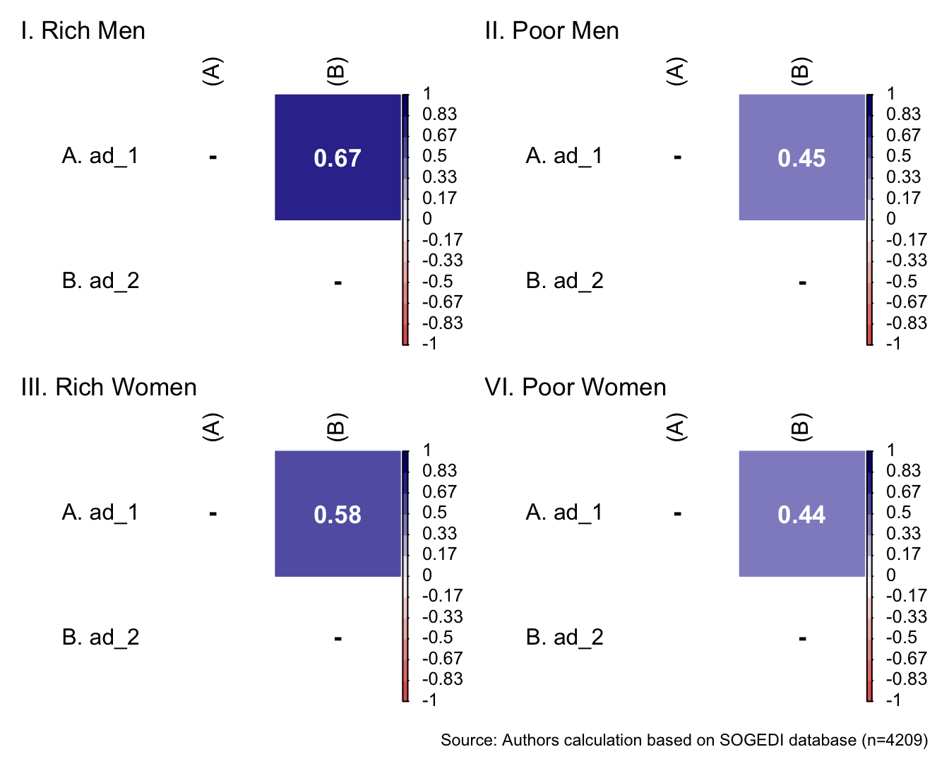
Reliability
5.4.10 Intergroup affect tendencies: contempt toward
We selected emotions that have been used in various studies that test the BIAS map from Cuddy et al. (2007).
Descriptive analysis
bind_rows(
psych::describe(db_rm[,c("co_1", "co_2")]) %>%
    as_tibble() %>%
    mutate(target = "Rich Men")
,
psych::describe(db_pm[,c("co_1", "co_2")]) %>%
    as_tibble() %>%
    mutate(target = "Poor Men")
,
psych::describe(db_rw[,c("co_1", "co_2")]) %>%
    as_tibble() %>%
    mutate(target = "Rich Women")
,
psych::describe(db_pw[,c("co_1", "co_2")]) %>%
    as_tibble() %>%
    mutate(target = "Poor Women")
) %>%
  mutate(vars = paste0("co_", vars)) %>%
  select(target, everything()) %>%
  group_by(target) %>%
  mutate(target = if_else(duplicated(target), NA, target)) %>%
kableExtra::kable(format = "markdown", digits = 3)| target | vars | n | mean | sd | median | trimmed | mad | min | max | range | skew | kurtosis | se |
|---|---|---|---|---|---|---|---|---|---|---|---|---|---|
| Rich Men | co_1 | 1043 | 2.062 | 1.500 | 1 | 1.790 | 0 | 1 | 7 | 6 | 1.341 | 0.903 | 0.046 |
| co_2 | 1043 | 2.228 | 1.567 | 1 | 1.968 | 0 | 1 | 7 | 6 | 1.099 | 0.251 | 0.049 | |
| Poor Men | co_1 | 1058 | 1.722 | 1.229 | 1 | 1.456 | 0 | 1 | 7 | 6 | 1.805 | 2.708 | 0.038 |
| co_2 | 1058 | 1.617 | 1.155 | 1 | 1.335 | 0 | 1 | 7 | 6 | 2.103 | 4.187 | 0.036 | |
| Rich Women | co_1 | 1056 | 1.770 | 1.333 | 1 | 1.481 | 0 | 1 | 7 | 6 | 1.790 | 2.481 | 0.041 |
| co_2 | 1056 | 1.886 | 1.381 | 1 | 1.618 | 0 | 1 | 7 | 6 | 1.556 | 1.638 | 0.043 | |
| Poor Women | co_1 | 1052 | 1.390 | 0.935 | 1 | 1.128 | 0 | 1 | 7 | 6 | 2.843 | 8.460 | 0.029 |
| co_2 | 1052 | 1.343 | 0.842 | 1 | 1.113 | 0 | 1 | 7 | 6 | 2.935 | 9.447 | 0.026 |
p1 <- wrap_elements(
    ~corrplot::corrplot(
      fit_correlations_pairwise(db_rm, c("co_1", "co_2")),
      method = "color",
      type = "upper",
      col = colorRampPalette(c("#E16462", "white", "#0D0887"))(12),
      tl.pos = "lt",
      tl.col = "black",
      addrect = 2,
      rect.col = "black",
      addCoef.col = "white",
      cl.cex = 0.8,
      cl.align.text = 'l',
      number.cex = 1.1,
      na.label = "-",
      bg = "white"
    )
  ) + labs(title = "I. Rich Men")


p2 <- wrap_elements(
    ~corrplot::corrplot(
      fit_correlations_pairwise(db_pm, c("co_1", "co_2")),
      method = "color",
      type = "upper",
      col = colorRampPalette(c("#E16462", "white", "#0D0887"))(12),
      tl.pos = "lt",
      tl.col = "black",
      addrect = 2,
      rect.col = "black",
      addCoef.col = "white",
      cl.cex = 0.8,
      cl.align.text = 'l',
      number.cex = 1.1,
      na.label = "-",
      bg = "white"
    )
  ) + labs(title = "II. Poor Men")

p3 <- wrap_elements(
    ~corrplot::corrplot(
      fit_correlations_pairwise(db_rw, c("co_1", "co_2")),
      method = "color",
      type = "upper",
      col = colorRampPalette(c("#E16462", "white", "#0D0887"))(12),
      tl.pos = "lt",
      tl.col = "black",
      addrect = 2,
      rect.col = "black",
      addCoef.col = "white",
      cl.cex = 0.8,
      cl.align.text = 'l',
      number.cex = 1.1,
      na.label = "-",
      bg = "white"
    )
  ) + labs(title = "III. Rich Women")

p4 <- wrap_elements(
    ~corrplot::corrplot(
      fit_correlations_pairwise(db_pw, c("co_1", "co_2")),
      method = "color",
      type = "upper",
      col = colorRampPalette(c("#E16462", "white", "#0D0887"))(12),
      tl.pos = "lt",
      tl.col = "black",
      addrect = 2,
      rect.col = "black",
      addCoef.col = "white",
      cl.cex = 0.8,
      cl.align.text = 'l',
      number.cex = 1.1,
      na.label = "-",
      bg = "white"
    )
  )+ labs(title = "VI. Poor Women")

a <- p1 + p2

b <- p3 + p4

a/b +
    plot_annotation(
      caption = paste0(
        "Source: Authors calculation based on SOGEDI",
        " database (n=", nrow(db_proc), ")"
      )
    )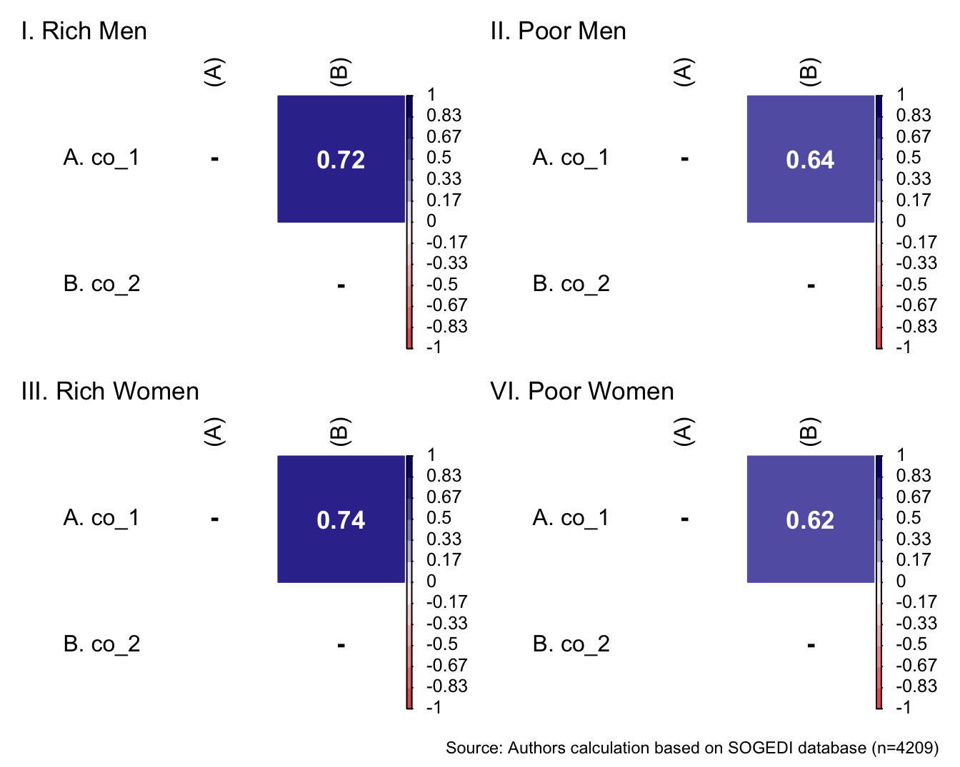
Reliability
5.4.11 Intergroup affect tendencies: envy toward
We selected emotions that have been used in various studies that test the BIAS map from Cuddy et al. (2007).
Descriptive analysis
bind_rows(
psych::describe(db_rm[,c("en_1", "en_2")]) %>%
    as_tibble() %>%
    mutate(target = "Rich Men")
,
psych::describe(db_pm[,c("en_1", "en_2")]) %>%
    as_tibble() %>%
    mutate(target = "Poor Men")
,
psych::describe(db_rw[,c("en_1", "en_2")]) %>%
    as_tibble() %>%
    mutate(target = "Rich Women")
,
psych::describe(db_pw[,c("en_1", "en_2")]) %>%
    as_tibble() %>%
    mutate(target = "Poor Women")
) %>%
  mutate(vars = paste0("en_", vars)) %>%
  select(target, everything()) %>%
  group_by(target) %>%
  mutate(target = if_else(duplicated(target), NA, target)) %>%
kableExtra::kable(format = "markdown", digits = 3)| target | vars | n | mean | sd | median | trimmed | mad | min | max | range | skew | kurtosis | se |
|---|---|---|---|---|---|---|---|---|---|---|---|---|---|
| Rich Men | en_1 | 1043 | 2.338 | 1.611 | 2 | 2.090 | 1.483 | 1 | 7 | 6 | 1.000 | 0.034 | 0.050 |
| en_2 | 1043 | 2.205 | 1.545 | 1 | 1.944 | 0.000 | 1 | 7 | 6 | 1.124 | 0.315 | 0.048 | |
| Poor Men | en_1 | 1058 | 1.509 | 1.050 | 1 | 1.232 | 0.000 | 1 | 7 | 6 | 2.323 | 5.264 | 0.032 |
| en_2 | 1058 | 1.491 | 1.036 | 1 | 1.217 | 0.000 | 1 | 7 | 6 | 2.354 | 5.404 | 0.032 | |
| Rich Women | en_1 | 1056 | 2.192 | 1.560 | 1 | 1.922 | 0.000 | 1 | 7 | 6 | 1.171 | 0.379 | 0.048 |
| en_2 | 1056 | 2.089 | 1.499 | 1 | 1.820 | 0.000 | 1 | 7 | 6 | 1.264 | 0.677 | 0.046 | |
| Poor Women | en_1 | 1052 | 1.355 | 0.920 | 1 | 1.102 | 0.000 | 1 | 7 | 6 | 3.218 | 11.559 | 0.028 |
| en_2 | 1052 | 1.375 | 0.975 | 1 | 1.101 | 0.000 | 1 | 7 | 6 | 3.126 | 10.292 | 0.030 |
p1 <- wrap_elements(
    ~corrplot::corrplot(
      fit_correlations_pairwise(db_rm, c("en_1", "en_2")),
      method = "color",
      type = "upper",
      col = colorRampPalette(c("#E16462", "white", "#0D0887"))(12),
      tl.pos = "lt",
      tl.col = "black",
      addrect = 2,
      rect.col = "black",
      addCoef.col = "white",
      cl.cex = 0.8,
      cl.align.text = 'l',
      number.cex = 1.1,
      na.label = "-",
      bg = "white"
    )
  ) + labs(title = "I. Rich Men")


p2 <- wrap_elements(
    ~corrplot::corrplot(
      fit_correlations_pairwise(db_pm, c("en_1", "en_2")),
      method = "color",
      type = "upper",
      col = colorRampPalette(c("#E16462", "white", "#0D0887"))(12),
      tl.pos = "lt",
      tl.col = "black",
      addrect = 2,
      rect.col = "black",
      addCoef.col = "white",
      cl.cex = 0.8,
      cl.align.text = 'l',
      number.cex = 1.1,
      na.label = "-",
      bg = "white"
    )
  ) + labs(title = "II. Poor Men")

p3 <- wrap_elements(
    ~corrplot::corrplot(
      fit_correlations_pairwise(db_rw, c("en_1", "en_2")),
      method = "color",
      type = "upper",
      col = colorRampPalette(c("#E16462", "white", "#0D0887"))(12),
      tl.pos = "lt",
      tl.col = "black",
      addrect = 2,
      rect.col = "black",
      addCoef.col = "white",
      cl.cex = 0.8,
      cl.align.text = 'l',
      number.cex = 1.1,
      na.label = "-",
      bg = "white"
    )
  ) + labs(title = "III. Rich Women")

p4 <- wrap_elements(
    ~corrplot::corrplot(
      fit_correlations_pairwise(db_pw, c("en_1", "en_2")),
      method = "color",
      type = "upper",
      col = colorRampPalette(c("#E16462", "white", "#0D0887"))(12),
      tl.pos = "lt",
      tl.col = "black",
      addrect = 2,
      rect.col = "black",
      addCoef.col = "white",
      cl.cex = 0.8,
      cl.align.text = 'l',
      number.cex = 1.1,
      na.label = "-",
      bg = "white"
    )
  )+ labs(title = "VI. Poor Women")

a <- p1 + p2

b <- p3 + p4

a/b +
    plot_annotation(
      caption = paste0(
        "Source: Authors calculation based on SOGEDI",
        " database (n=", nrow(db_proc), ")"
      )
    )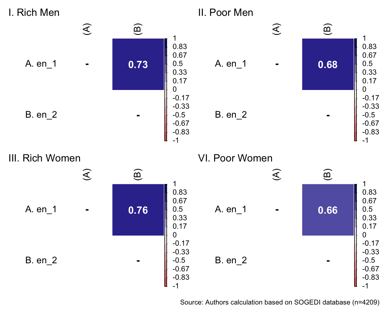
Reliability
5.4.12 Intergroup affect tendencies: pity toward
We selected emotions that have been used in various studies that test the BIAS map from Cuddy et al. (2007).
Descriptive analysis
bind_rows(
psych::describe(db_rm[,c("pi_1", "pi_2")]) %>%
    as_tibble() %>%
    mutate(target = "Rich Men")
,
psych::describe(db_pm[,c("pi_1", "pi_2")]) %>%
    as_tibble() %>%
    mutate(target = "Poor Men")
,
psych::describe(db_rw[,c("pi_1", "pi_2")]) %>%
    as_tibble() %>%
    mutate(target = "Rich Women")
,
psych::describe(db_pw[,c("pi_1", "pi_2")]) %>%
    as_tibble() %>%
    mutate(target = "Poor Women")
) %>%
  mutate(vars = paste0("pi_", vars)) %>%
  select(target, everything()) %>%
  group_by(target) %>%
  mutate(target = if_else(duplicated(target), NA, target)) %>%
kableExtra::kable(format = "markdown", digits = 3)| target | vars | n | mean | sd | median | trimmed | mad | min | max | range | skew | kurtosis | se |
|---|---|---|---|---|---|---|---|---|---|---|---|---|---|
| Rich Men | pi_1 | 1043 | 2.062 | 1.449 | 1 | 1.814 | 0.000 | 1 | 7 | 6 | 1.265 | 0.734 | 0.045 |
| pi_2 | 1043 | 2.213 | 1.459 | 2 | 2.019 | 1.483 | 1 | 7 | 6 | 0.961 | 0.022 | 0.045 | |
| Poor Men | pi_1 | 1058 | 3.336 | 1.895 | 3 | 3.226 | 2.965 | 1 | 7 | 6 | 0.202 | -1.111 | 0.058 |
| pi_2 | 1058 | 4.006 | 1.826 | 4 | 4.007 | 1.483 | 1 | 7 | 6 | -0.162 | -0.855 | 0.056 | |
| Rich Women | pi_1 | 1056 | 1.959 | 1.435 | 1 | 1.696 | 0.000 | 1 | 7 | 6 | 1.451 | 1.309 | 0.044 |
| pi_2 | 1056 | 2.261 | 1.540 | 2 | 2.026 | 1.483 | 1 | 7 | 6 | 1.049 | 0.238 | 0.047 | |
| Poor Women | pi_1 | 1052 | 3.199 | 1.910 | 3 | 3.053 | 2.965 | 1 | 7 | 6 | 0.320 | -1.081 | 0.059 |
| pi_2 | 1052 | 4.108 | 1.880 | 4 | 4.135 | 1.483 | 1 | 7 | 6 | -0.176 | -0.943 | 0.058 |
p1 <- wrap_elements(
    ~corrplot::corrplot(
      fit_correlations_pairwise(db_rm, c("pi_1", "pi_2")),
      method = "color",
      type = "upper",
      col = colorRampPalette(c("#E16462", "white", "#0D0887"))(12),
      tl.pos = "lt",
      tl.col = "black",
      addrect = 2,
      rect.col = "black",
      addCoef.col = "white",
      cl.cex = 0.8,
      cl.align.text = 'l',
      number.cex = 1.1,
      na.label = "-",
      bg = "white"
    )
  ) + labs(title = "I. Rich Men")


p2 <- wrap_elements(
    ~corrplot::corrplot(
      fit_correlations_pairwise(db_pm, c("pi_1", "pi_2")),
      method = "color",
      type = "upper",
      col = colorRampPalette(c("#E16462", "white", "#0D0887"))(12),
      tl.pos = "lt",
      tl.col = "black",
      addrect = 2,
      rect.col = "black",
      addCoef.col = "white",
      cl.cex = 0.8,
      cl.align.text = 'l',
      number.cex = 1.1,
      na.label = "-",
      bg = "white"
    )
  ) + labs(title = "II. Poor Men")

p3 <- wrap_elements(
    ~corrplot::corrplot(
      fit_correlations_pairwise(db_rw, c("pi_1", "pi_2")),
      method = "color",
      type = "upper",
      col = colorRampPalette(c("#E16462", "white", "#0D0887"))(12),
      tl.pos = "lt",
      tl.col = "black",
      addrect = 2,
      rect.col = "black",
      addCoef.col = "white",
      cl.cex = 0.8,
      cl.align.text = 'l',
      number.cex = 1.1,
      na.label = "-",
      bg = "white"
    )
  ) + labs(title = "III. Rich Women")

p4 <- wrap_elements(
    ~corrplot::corrplot(
      fit_correlations_pairwise(db_pw, c("pi_1", "pi_2")),
      method = "color",
      type = "upper",
      col = colorRampPalette(c("#E16462", "white", "#0D0887"))(12),
      tl.pos = "lt",
      tl.col = "black",
      addrect = 2,
      rect.col = "black",
      addCoef.col = "white",
      cl.cex = 0.8,
      cl.align.text = 'l',
      number.cex = 1.1,
      na.label = "-",
      bg = "white"
    )
  )+ labs(title = "VI. Poor Women")

a <- p1 + p2

b <- p3 + p4

a/b +
    plot_annotation(
      caption = paste0(
        "Source: Authors calculation based on SOGEDI",
        " database (n=", nrow(db_proc), ")"
      )
    )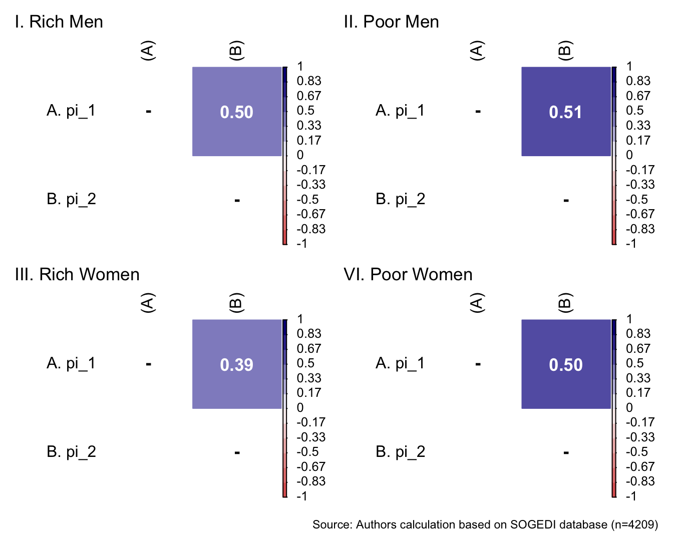
Reliability
5.4.13 Greedy dispositions
Exploratory items were developed by the project team.
Descriptive analysis
bind_rows(
psych::describe(db_rm[,c("greedy_1", "greedy_2", "greedy_3")]) %>%
    as_tibble() %>%
    mutate(target = "Rich Men")
,
psych::describe(db_rw[,c("greedy_1", "greedy_2", "greedy_3")]) %>%
    as_tibble() %>%
    mutate(target = "Rich Women")
) %>%
  mutate(vars = paste0("greedy_", vars)) %>%
  select(target, everything()) %>%
  group_by(target) %>%
  mutate(target = if_else(duplicated(target), NA, target)) %>%
kableExtra::kable(format = "markdown", digits = 3)| target | vars | n | mean | sd | median | trimmed | mad | min | max | range | skew | kurtosis | se |
|---|---|---|---|---|---|---|---|---|---|---|---|---|---|
| Rich Men | greedy_1 | 1043 | 5.354 | 1.716 | 6 | 5.604 | 1.483 | 1 | 7 | 6 | -0.920 | 0.073 | 0.053 |
| greedy_2 | 1043 | 5.021 | 1.644 | 5 | 5.177 | 1.483 | 1 | 7 | 6 | -0.602 | -0.292 | 0.051 | |
| greedy_3 | 1043 | 5.057 | 1.630 | 5 | 5.208 | 1.483 | 1 | 7 | 6 | -0.555 | -0.350 | 0.050 | |
| Rich Women | greedy_1 | 1056 | 4.644 | 1.831 | 5 | 4.793 | 1.483 | 1 | 7 | 6 | -0.403 | -0.675 | 0.056 |
| greedy_2 | 1056 | 4.445 | 1.733 | 4 | 4.525 | 1.483 | 1 | 7 | 6 | -0.266 | -0.657 | 0.053 | |
| greedy_3 | 1056 | 4.929 | 1.603 | 5 | 5.052 | 1.483 | 1 | 7 | 6 | -0.405 | -0.401 | 0.049 |
p1 <- wrap_elements(
    ~corrplot::corrplot(
      fit_correlations(db_rm, c("greedy_1", "greedy_2", "greedy_3")),
      method = "color",
      type = "upper",
      col = colorRampPalette(c("#E16462", "white", "#0D0887"))(12),
      tl.pos = "lt",
      tl.col = "black",
      addrect = 2,
      rect.col = "black",
      addCoef.col = "white",
      cl.cex = 0.8,
      cl.align.text = 'l',
      number.cex = 1.1,
      na.label = "-",
      bg = "white"
    )
  ) + labs(title = "I. Rich Men")


p2 <- wrap_elements(
    ~corrplot::corrplot(
      fit_correlations(db_rw, c("greedy_1", "greedy_2", "greedy_3")),
      method = "color",
      type = "upper",
      col = colorRampPalette(c("#E16462", "white", "#0D0887"))(12),
      tl.pos = "lt",
      tl.col = "black",
      addrect = 2,
      rect.col = "black",
      addCoef.col = "white",
      cl.cex = 0.8,
      cl.align.text = 'l',
      number.cex = 1.1,
      na.label = "-",
      bg = "white"
    )
  ) + labs(title = "II. Rich Women")


p1/p2 +
    plot_annotation(
      caption = paste0(
        "Source: Authors calculation based on SOGEDI",
        " database (n=1043)"
      )
    )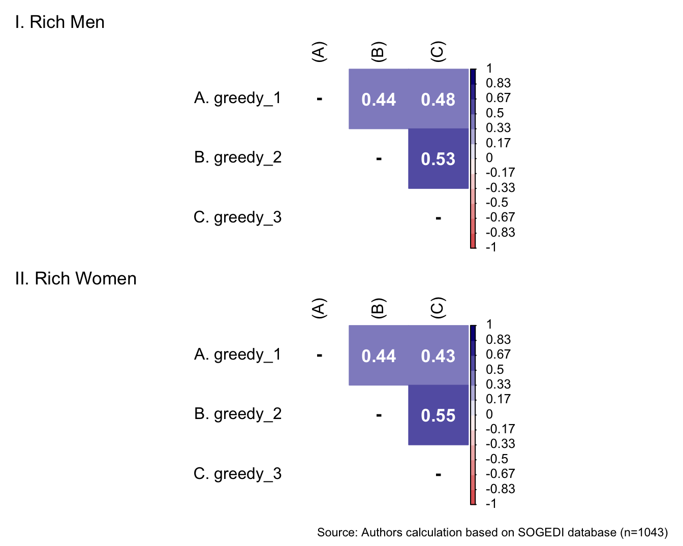
Reliability
mi_variable <- "greedy"
result2 <- alphas(db_proc, c("greedy_1", "greedy_2", "greedy_3"), mi_variable)

result2$raw_alpha
[1] 0.7350066result2$new_var_summary Min. 1st Qu. Median Mean 3rd Qu. Max. NA's
1.000 4.000 5.000 4.907 6.000 7.000 2110 Confirmatory factor analysis
Mardia’s test for evaluate multivariate normality for each target.
mardia(db_rm[,c("greedy_1", "greedy_2", "greedy_3")],
       na.rm = T, plot=T)
Call: mardia(x = db_rm[, c(“greedy_1”, “greedy_2”, “greedy_3”)], na.rm = T, plot = T)
Mardia tests of multivariate skew and kurtosis Use describe(x) the to get univariate tests n.obs = 1043 num.vars = 3 b1p = 2.25 skew = 391.8 with probability <= 0.0000000000000000000000000000000000000000000000000000000000000000000000000000052 small sample skew = 393.5 with probability <= 0.0000000000000000000000000000000000000000000000000000000000000000000000000000023 b2p = 20.86 kurtosis = 17.28 with probability <= 0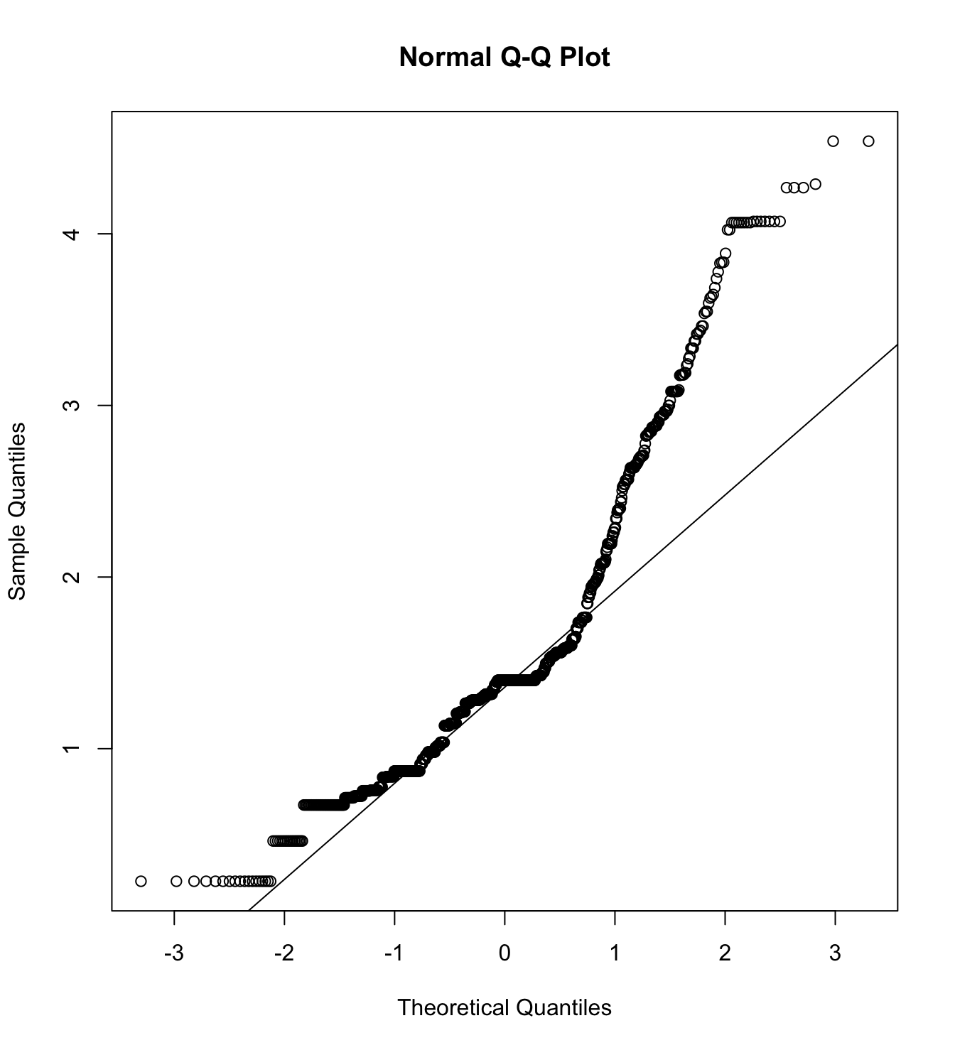
We first specify the factorial structure of the items, then fit models using a robust maximum likelihood estimator for the entire sample as well as for each country individually. The goodnes of fit indicators are shown.
# model
model_cfa <- '
  greedy_disp =~ greedy_1 + greedy_2 + greedy_3
   '

# estimation
# overall
m12_cfa_rm <- cfa(model = model_cfa,
              data = subset(db_proc, target == "Rich.Men"),
              estimator = "MLR",
              ordered = F,
              std.lv = F)

m12_cfa_rw <- cfa(model = model_cfa,
              data = subset(db_proc, target == "Rich.Women"),
              estimator = "MLR",
              ordered = F,
              std.lv = F)

# argentina
m12_cfa_rm_arg <- cfa(model = model_cfa,
                 data = subset(db_proc, group == "1.Rich.Men"),
                 estimator = "MLR",
                 ordered = F,
                 std.lv = F)

m12_cfa_rw_arg <- cfa(model = model_cfa,
                 data = subset(db_proc, group == "1.Rich.Women"),
                 estimator = "MLR",
                 ordered = F,
                 std.lv = F)

# chile
m12_cfa_rm_cl <- cfa(model = model_cfa,
                     data = subset(db_proc, group == "3.Rich.Men"),
                     estimator = "MLR",
                     ordered = F,
                     std.lv = F)


m12_cfa_rw_cl <- cfa(model = model_cfa,
                     data = subset(db_proc, group == "3.Rich.Women"),
                     estimator = "MLR",
                     ordered = F,
                     std.lv = F)

# colombia
m12_cfa_rm_col <- cfa(model = model_cfa,
                     data = subset(db_proc, group == "4.Rich.Men"),
                     estimator = "MLR",
                     ordered = F,
                     std.lv = F)


m12_cfa_rw_col <- cfa(model = model_cfa,
                     data = subset(db_proc, group == "4.Rich.Women"),
                     estimator = "MLR",
                     ordered = F,
                     std.lv = F)


# españa
m12_cfa_rm_esp <- cfa(model = model_cfa,
                     data = subset(db_proc, group == "9.Rich.Men"),
                     estimator = "MLR",
                     ordered = F,
                     std.lv = F)


m12_cfa_rw_esp <- cfa(model = model_cfa,
                     data = subset(db_proc, group == "9.Rich.Women"),
                     estimator = "MLR",
                     ordered = F,
                     std.lv = F)


# mexico
m12_cfa_rm_mex <- cfa(model = model_cfa,
                     data = subset(db_proc, group == "13.Rich.Men"),
                     estimator = "MLR",
                     ordered = F,
                     std.lv = F)


m12_cfa_rw_mex <- cfa(model = model_cfa,
                     data = subset(db_proc, group == "13.Rich.Women"),
                     estimator = "MLR",
                     ordered = F,
                     std.lv = F)
colnames_fit <- c("","Target","$N$","Estimator","$\\chi^2$ (df)","CFI","TLI","RMSEA 90% CI [Lower-Upper]", "SRMR", "AIC")
bind_rows(
cfa_tab_fit(
models = list(m12_cfa_rm, m12_cfa_rm_arg, m12_cfa_rm_cl, m12_cfa_rm_col, m12_cfa_rm_esp, m12_cfa_rm_mex),
country_names = c("Overall scores", "Argentina", "Chile", "Colombia", "Spain", "México")
)$sum_fit %>%
mutate(target = "Rich Men")
,
cfa_tab_fit(
models = list(m12_cfa_rw, m12_cfa_rw_arg, m12_cfa_rw_cl, m12_cfa_rw_col, m12_cfa_rw_esp, m12_cfa_rw_mex),
country_names = c("Overall scores", "Argentina", "Chile", "Colombia", "Spain", "México")
)$sum_fit %>%
mutate(target = "Rich Women")
) %>%
select(country, target, everything()) %>%
mutate(country = factor(country, levels = c("Overall scores", "Argentina", "Chile", "Colombia", "Spain", "México"))) %>%
group_by(country) %>%
arrange(country) %>%
mutate(country = if_else(duplicated(country), NA, country)) %>%
kableExtra::kable(
format = "markdown",
digits = 3,
booktabs = TRUE,
col.names = colnames_fit,
caption = NULL
) %>%
kableExtra::kable_styling(
full_width = TRUE,
font_size = 11,
latex_options = "HOLD_position",
bootstrap_options = c("striped", "bordered")
) %>%
kableExtra::collapse_rows(columns = 1)| Target | \(N\) | Estimator | \(\chi^2\) (df) | CFI | TLI | RMSEA 90% CI [Lower-Upper] | SRMR | AIC | |
|---|---|---|---|---|---|---|---|---|---|
| Overall scores | Rich Men | 1043 | ML | 0 (0) | 1 | 1 | 0 [0-0] | 0 | 11385.705 |
| Rich Women | 1056 | ML | 0 (0) | 1 | 1 | 0 [0-0] | 0 | 11755.575 | |
| Argentina | Rich Men | 216 | ML | 0 (0) | 1 | 1 | 0 [0-0] | 0 | 2339.979 |
| Rich Women | 207 | ML | 0 (0) | 1 | 1 | 0 [0-0] | 0 | 2300.126 | |
| Chile | Rich Men | 217 | ML | 0 (0) | 1 | 1 | 0 [0-0] | 0 | 2407.232 |
| Rich Women | 223 | ML | 0 (0) | 1 | 1 | 0 [0-0] | 0 | 2456.741 | |
| Colombia | Rich Men | 206 | ML | 0 (0) | 1 | 1 | 0 [0-0] | 0 | 2294.079 |
| Rich Women | 199 | ML | 0 (0) | 1 | 1 | 0 [0-0] | 0 | 2323.775 | |
| Spain | Rich Men | 195 | ML | 0 (0) | 1 | 1 | 0 [0-0] | 0 | 1972.255 |
| Rich Women | 212 | ML | 0 (0) | 1 | 1 | 0 [0-0] | 0 | 2138.112 | |
| México | Rich Men | 209 | ML | 0 (0) | 1 | 1 | 0 [0-0] | 0 | 2325.053 |
| Rich Women | 215 | ML | 0 (0) | 1 | 1 | 0 [0-0] | 0 | 2432.016 |
5.4.14 Punishment rich
Exploratory items were developed by the project team.
Descriptive analysis
bind_rows(
psych::describe(db_rm[,c("punish_1", "punish_2", "punish_3")]) %>%
    as_tibble() %>%
    mutate(target = "Rich Men")
,
psych::describe(db_rw[,c("punish_1", "punish_2", "punish_3")]) %>%
    as_tibble() %>%
    mutate(target = "Rich Women")
) %>%
  mutate(vars = paste0("punish_", vars)) %>%
  select(target, everything()) %>%
  group_by(target) %>%
  mutate(target = if_else(duplicated(target), NA, target)) %>%
kableExtra::kable(format = "markdown", digits = 3)| target | vars | n | mean | sd | median | trimmed | mad | min | max | range | skew | kurtosis | se |
|---|---|---|---|---|---|---|---|---|---|---|---|---|---|
| Rich Men | punish_1 | 1043 | 5.415 | 1.932 | 6 | 5.739 | 1.483 | 1 | 7 | 6 | -1.011 | -0.167 | 0.060 |
| punish_2 | 1043 | 6.066 | 1.493 | 7 | 6.376 | 0.000 | 1 | 7 | 6 | -1.662 | 2.072 | 0.046 | |
| punish_3 | 1043 | 6.212 | 1.394 | 7 | 6.521 | 0.000 | 1 | 7 | 6 | -1.800 | 2.464 | 0.043 | |
| Rich Women | punish_1 | 1056 | 4.420 | 2.219 | 4 | 4.524 | 2.965 | 1 | 7 | 6 | -0.290 | -1.292 | 0.068 |
| punish_2 | 1056 | 5.648 | 1.784 | 7 | 5.975 | 0.000 | 1 | 7 | 6 | -1.210 | 0.447 | 0.055 | |
| punish_3 | 1056 | 6.127 | 1.522 | 7 | 6.466 | 0.000 | 1 | 7 | 6 | -1.817 | 2.524 | 0.047 |
p1 <- wrap_elements(
    ~corrplot::corrplot(
      fit_correlations(db_rm, c("punish_1", "punish_2", "punish_3")),
      method = "color",
      type = "upper",
      col = colorRampPalette(c("#E16462", "white", "#0D0887"))(12),
      tl.pos = "lt",
      tl.col = "black",
      addrect = 2,
      rect.col = "black",
      addCoef.col = "white",
      cl.cex = 0.8,
      cl.align.text = 'l',
      number.cex = 1.1,
      na.label = "-",
      bg = "white"
    )
  ) + labs(title = "I. Rich Men")


p2 <- wrap_elements(
    ~corrplot::corrplot(
      fit_correlations(db_rw, c("punish_1", "punish_2", "punish_3")),
      method = "color",
      type = "upper",
      col = colorRampPalette(c("#E16462", "white", "#0D0887"))(12),
      tl.pos = "lt",
      tl.col = "black",
      addrect = 2,
      rect.col = "black",
      addCoef.col = "white",
      cl.cex = 0.8,
      cl.align.text = 'l',
      number.cex = 1.1,
      na.label = "-",
      bg = "white"
    )
  ) + labs(title = "II. Rich Women")


p1/p2 +
    plot_annotation(
      caption = paste0(
        "Source: Authors calculation based on SOGEDI",
        " database (n=1043)"
      )
    )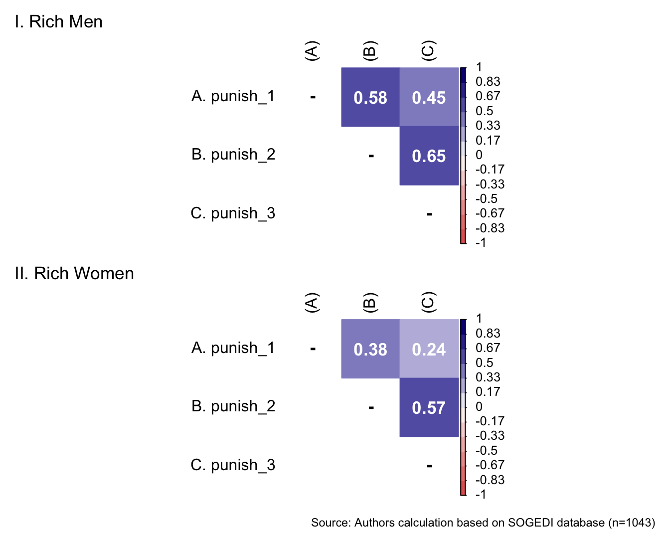
Reliability
mi_variable <- "punish"
result2 <- alphas(db_proc, c("punish_1", "punish_2", "punish_3"), mi_variable)

result2$raw_alpha
[1] 0.7030876result2$new_var_summary Min. 1st Qu. Median Mean 3rd Qu. Max. NA's
1.000 5.000 6.000 5.646 7.000 7.000 2110 Confirmatory factor analysis
Mardia’s test for evaluate multivariate normality for each target.
mardia(db_rm[,c("punish_1", "punish_2", "punish_3")],
       na.rm = T, plot=T)
Call: mardia(x = db_rm[, c(“punish_1”, “punish_2”, “punish_3”)], na.rm = T, plot = T)
Mardia tests of multivariate skew and kurtosis Use describe(x) the to get univariate tests n.obs = 1043 num.vars = 3 b1p = 9.22 skew = 1602.41 with probability <= 0 small sample skew = 1609.34 with probability <= 0 b2p = 28.41 kurtosis = 39.53 with probability <= 0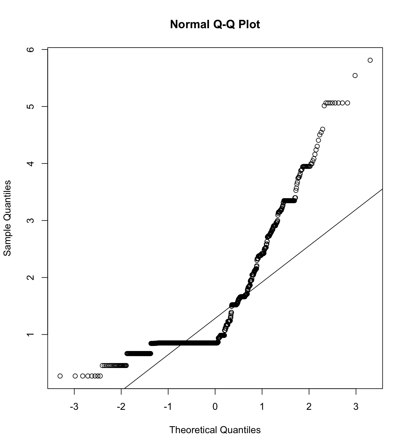
We first specify the factorial structure of the items, then fit models using a robust maximum likelihood estimator for the entire sample as well as for each country individually. The goodnes of fit indicators are shown.
# model
model_cfa <- '
  punishment =~ punish_1 + punish_2 + punish_3
   '

# estimation
# overall
m13_cfa_rm <- cfa(model = model_cfa,
              data = subset(db_proc, target == "Rich.Men"),
              estimator = "MLR",
              ordered = F,
              std.lv = F)

m13_cfa_rw <- cfa(model = model_cfa,
              data = subset(db_proc, target == "Rich.Women"),
              estimator = "MLR",
              ordered = F,
              std.lv = F)

# argentina
m13_cfa_rm_arg <- cfa(model = model_cfa,
                 data = subset(db_proc, group == "1.Rich.Men"),
                 estimator = "MLR",
                 ordered = F,
                 std.lv = F)

m13_cfa_rw_arg <- cfa(model = model_cfa,
                 data = subset(db_proc, group == "1.Rich.Women"),
                 estimator = "MLR",
                 ordered = F,
                 std.lv = F)

# chile
m13_cfa_rm_cl <- cfa(model = model_cfa,
                     data = subset(db_proc, group == "3.Rich.Men"),
                     estimator = "MLR",
                     ordered = F,
                     std.lv = F)


m13_cfa_rw_cl <- cfa(model = model_cfa,
                     data = subset(db_proc, group == "3.Rich.Women"),
                     estimator = "MLR",
                     ordered = F,
                     std.lv = F)

# colombia
m13_cfa_rm_col <- cfa(model = model_cfa,
                     data = subset(db_proc, group == "4.Rich.Men"),
                     estimator = "MLR",
                     ordered = F,
                     std.lv = F)


m13_cfa_rw_col <- cfa(model = model_cfa,
                     data = subset(db_proc, group == "4.Rich.Women"),
                     estimator = "MLR",
                     ordered = F,
                     std.lv = F)


# españa
m13_cfa_rm_esp <- cfa(model = model_cfa,
                     data = subset(db_proc, group == "9.Rich.Men"),
                     estimator = "MLR",
                     ordered = F,
                     std.lv = F)


m13_cfa_rw_esp <- cfa(model = model_cfa,
                     data = subset(db_proc, group == "9.Rich.Women"),
                     estimator = "MLR",
                     ordered = F,
                     std.lv = F)


# mexico
m13_cfa_rm_mex <- cfa(model = model_cfa,
                     data = subset(db_proc, group == "13.Rich.Men"),
                     estimator = "MLR",
                     ordered = F,
                     std.lv = F)


m13_cfa_rw_mex <- cfa(model = model_cfa,
                     data = subset(db_proc, group == "13.Rich.Women"),
                     estimator = "MLR",
                     ordered = F,
                     std.lv = F)
colnames_fit <- c("","Target","$N$","Estimator","$\\chi^2$ (df)","CFI","TLI","RMSEA 90% CI [Lower-Upper]", "SRMR", "AIC")
bind_rows(
cfa_tab_fit(
models = list(m13_cfa_rm, m13_cfa_rm_arg, m13_cfa_rm_cl, m13_cfa_rm_col, m13_cfa_rm_esp, m13_cfa_rm_mex),
country_names = c("Overall scores", "Argentina", "Chile", "Colombia", "Spain", "México")
)$sum_fit %>%
mutate(target = "Rich Men")
,
cfa_tab_fit(
models = list(m13_cfa_rw, m13_cfa_rw_arg, m13_cfa_rw_cl, m13_cfa_rw_col, m13_cfa_rw_esp, m13_cfa_rw_mex),
country_names = c("Overall scores", "Argentina", "Chile", "Colombia", "Spain", "México")
)$sum_fit %>%
mutate(target = "Rich Women")
) %>%
select(country, target, everything()) %>%
mutate(country = factor(country, levels = c("Overall scores", "Argentina", "Chile", "Colombia", "Spain", "México"))) %>%
group_by(country) %>%
arrange(country) %>%
mutate(country = if_else(duplicated(country), NA, country)) %>%
kableExtra::kable(
format = "markdown",
digits = 3,
booktabs = TRUE,
col.names = colnames_fit,
caption = NULL
) %>%
kableExtra::kable_styling(
full_width = TRUE,
font_size = 11,
latex_options = "HOLD_position",
bootstrap_options = c("striped", "bordered")
) %>%
kableExtra::collapse_rows(columns = 1)| Target | \(N\) | Estimator | \(\chi^2\) (df) | CFI | TLI | RMSEA 90% CI [Lower-Upper] | SRMR | AIC | |
|---|---|---|---|---|---|---|---|---|---|
| Overall scores | Rich Men | 1043 | ML | 0 (0) | 1 | 1 | 0 [0-0] | 0 | 10781.580 |
| Rich Women | 1056 | ML | 0 (0) | 1 | 1 | 0 [0-0] | 0 | 12218.219 | |
| Argentina | Rich Men | 216 | ML | 0 (0) | 1 | 1 | 0 [0-0] | 0 | 2329.549 |
| Rich Women | 207 | ML | 0 (0) | 1 | 1 | 0 [0-0] | 0 | 2491.412 | |
| Chile | Rich Men | 217 | ML | 0 (0) | 1 | 1 | 0 [0-0] | 0 | 2074.506 |
| Rich Women | 223 | ML | 0 (0) | 1 | 1 | 0 [0-0] | 0 | 2539.111 | |
| Colombia | Rich Men | 206 | ML | 0 (0) | 1 | 1 | 0 [0-0] | 0 | 2202.810 |
| Rich Women | 199 | ML | 0 (0) | 1 | 1 | 0 [0-0] | 0 | 2285.530 | |
| Spain | Rich Men | 195 | ML | 0 (0) | 1 | 1 | 0 [0-0] | 0 | 1929.482 |
| Rich Women | 212 | ML | 0 (0) | 1 | 1 | 0 [0-0] | 0 | 2346.049 | |
| México | Rich Men | 209 | ML | 0 (0) | 1 | 1 | 0 [0-0] | 0 | 2142.628 |
| Rich Women | 215 | ML | 0 (0) | 1 | 1 | 0 [0-0] | 0 | 2524.644 |
5.5 Block 5. Atributions
5.5.1 Atributtions about poverty
We use the items with higher loading on each factor from the Spanish adaptation of the poverty and wealth attributions scales based on Sainz et al. (2023).
Descriptive analysis
bind_rows(
psych::describe(db_pm[,c("ex_po_1", "ex_po_2", "in_po_1", "in_po_2")]) %>%
    as_tibble() %>%
    mutate(target = "Poor Men")
,
psych::describe(db_pw[,c("ex_po_1", "ex_po_2", "in_po_1", "in_po_2")]) %>%
    as_tibble() %>%
    mutate(target = "Poor Women")
) %>%
  mutate(vars = case_when(vars <= 2 ~ paste0("ex_po_", vars),
                          vars >= 3 ~ paste0("in_po_", vars))) %>%
  select(target, everything()) %>%
  group_by(target) %>%
  mutate(target = if_else(duplicated(target), NA, target)) %>%
kableExtra::kable(format = "markdown", digits = 3)| target | vars | n | mean | sd | median | trimmed | mad | min | max | range | skew | kurtosis | se |
|---|---|---|---|---|---|---|---|---|---|---|---|---|---|
| Poor Men | ex_po_1 | 1058 | 5.141 | 1.608 | 5 | 5.311 | 1.483 | 1 | 7 | 6 | -0.657 | -0.172 | 0.049 |
| ex_po_2 | 1058 | 4.917 | 1.746 | 5 | 5.091 | 1.483 | 1 | 7 | 6 | -0.551 | -0.518 | 0.054 | |
| in_po_3 | 1058 | 4.128 | 1.786 | 4 | 4.159 | 1.483 | 1 | 7 | 6 | -0.082 | -0.841 | 0.055 | |
| in_po_4 | 1058 | 4.421 | 1.930 | 4 | 4.525 | 2.965 | 1 | 7 | 6 | -0.303 | -0.951 | 0.059 | |
| Poor Women | ex_po_1 | 1052 | 5.201 | 1.646 | 5 | 5.391 | 1.483 | 1 | 7 | 6 | -0.746 | -0.123 | 0.051 |
| ex_po_2 | 1052 | 4.971 | 1.740 | 5 | 5.156 | 1.483 | 1 | 7 | 6 | -0.617 | -0.456 | 0.054 | |
| in_po_3 | 1052 | 3.557 | 1.844 | 4 | 3.468 | 1.483 | 1 | 7 | 6 | 0.199 | -0.923 | 0.057 | |
| in_po_4 | 1052 | 4.211 | 1.982 | 4 | 4.264 | 2.965 | 1 | 7 | 6 | -0.176 | -1.091 | 0.061 |
p1 <- wrap_elements(
    ~corrplot::corrplot(
      fit_correlations_pairwise(db_pm, c("ex_po_1", "ex_po_2", "in_po_1", "in_po_2")),
      method = "color",
      type = "upper",
      col = colorRampPalette(c("#E16462", "white", "#0D0887"))(12),
      tl.pos = "lt",
      tl.col = "black",
      addrect = 2,
      rect.col = "black",
      addCoef.col = "white",
      cl.cex = 0.8,
      cl.align.text = 'l',
      number.cex = 1.1,
      na.label = "-",
      bg = "white"
    )
  ) + labs(title = "I. Poor Men")


p2 <- wrap_elements(
    ~corrplot::corrplot(
      fit_correlations_pairwise(db_pw, c("ex_po_1", "ex_po_2", "in_po_1", "in_po_2")),
      method = "color",
      type = "upper",
      col = colorRampPalette(c("#E16462", "white", "#0D0887"))(12),
      tl.pos = "lt",
      tl.col = "black",
      addrect = 2,
      rect.col = "black",
      addCoef.col = "white",
      cl.cex = 0.8,
      cl.align.text = 'l',
      number.cex = 1.1,
      na.label = "-",
      bg = "white"
    )
  ) + labs(title = "II. Poor Women")


p1/p2 +
    plot_annotation(
      caption = paste0(
        "Source: Authors calculation based on SOGEDI",
        " database (n=1043)"
      )
    )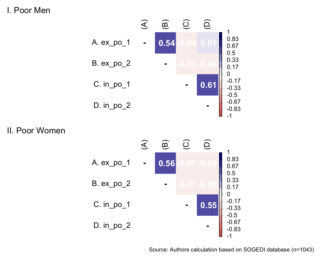
Reliability
mi_variable <- "ex_atri_po"
result2 <- alphas(db_proc, c("ex_po_1", "ex_po_2"), mi_variable)

result2$raw_alpha
[1] 0.709259result2$new_var_summary Min. 1st Qu. Median Mean 3rd Qu. Max. NA's
1.000 4.000 5.000 5.057 6.500 7.000 2099 mi_variable <- "in_atri_po"
result3 <- alphas(db_proc, c("in_po_1", "in_po_2"), mi_variable)
result3$raw_alpha[1] 0.7319118result3$new_var_summary Min. 1st Qu. Median Mean 3rd Qu. Max. NA's
1.00 3.00 4.00 4.08 5.50 7.00 2099 Confirmatory factor analysis
Mardia’s test for evaluate multivariate normality for each target.
mardia(db_pm[,c("ex_po_1", "ex_po_2", "in_po_1", "in_po_2")],
       na.rm = T, plot=T)
Call: mardia(x = db_pm[, c(“ex_po_1”, “ex_po_2”, “in_po_1”, “in_po_2”)], na.rm = T, plot = T)
Mardia tests of multivariate skew and kurtosis Use describe(x) the to get univariate tests n.obs = 1058 num.vars = 4 b1p = 1.61 skew = 283.02 with probability <= 0.0000000000000000000000000000000000000000000000023 small sample skew = 284.14 with probability <= 0.0000000000000000000000000000000000000000000000014 b2p = 27.29 kurtosis = 7.73 with probability <= 0.000000000000011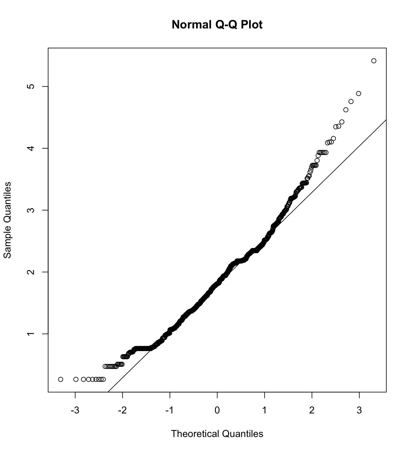
mardia(db_pw[,c("ex_po_1", "ex_po_2", "in_po_1", "in_po_2")],
       na.rm = T, plot=T)
Call: mardia(x = db_pw[, c(“ex_po_1”, “ex_po_2”, “in_po_1”, “in_po_2”)], na.rm = T, plot = T)
Mardia tests of multivariate skew and kurtosis Use describe(x) the to get univariate tests n.obs = 1052 num.vars = 4 b1p = 1.5 skew = 263.86 with probability <= 0.000000000000000000000000000000000000000000018 small sample skew = 264.91 with probability <= 0.000000000000000000000000000000000000000000011 b2p = 26.82 kurtosis = 6.61 with probability <= 0.000000000039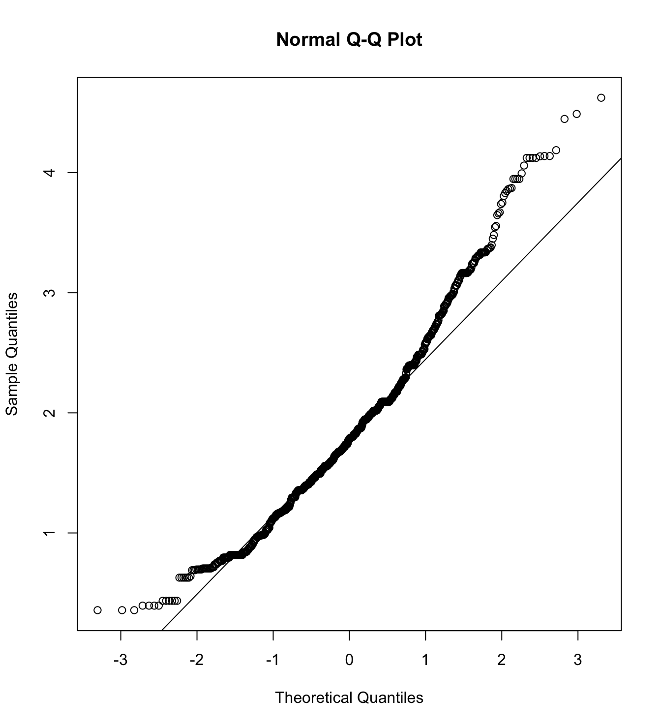
We first specify the factorial structure of the items, then fit models using a robust maximum likelihood estimator for the entire sample as well as for each country individually. The goodness of fit indicators are shown.
# model
#model_cfa <- '
#  external_atri_po =~ ex_po_1 + ex_po_2
#  internal_atri_po =~ in_po_1 + in_po_2
#'
#
## estimation
## overall
#m14_cfa_pm <- cfa(model = model_cfa,
#              data = subset(db_proc, target == "Poor.Men"),
#              estimator = "MLR",
#              ordered = F,
#              std.lv = F)
#
#m14_cfa_pw <- cfa(model = model_cfa,
#              data = subset(db_proc, target == "Poor.Women"),
#              estimator = "MLR",
#              ordered = F,
#              std.lv = F)
#
## argentina
#m14_cfa_pm_arg <- cfa(model = model_cfa,
#                 data = subset(db_proc, group == "1.Poor.Men"),
#                 estimator = "MLR",
#                 ordered = F,
#                 std.lv = F)
#
#m14_cfa_pw_arg <- cfa(model = model_cfa,
#                 data = subset(db_proc, group == "1.Poor.Women"),
#                 estimator = "MLR",
#                 ordered = F,
#                 std.lv = F)
#
## chile
#m14_cfa_pm_cl <- cfa(model = model_cfa,
#                     data = subset(db_proc, group == "3.Poor.Men"),
#                     estimator = "MLR",
#                     ordered = F,
#                     std.lv = F)
#
#
#m14_cfa_pw_cl <- cfa(model = model_cfa,
#                     data = subset(db_proc, group == "3.Poor.Women"),
#                     estimator = "MLR",
#                     ordered = F,
#                     std.lv = F)
#
## colombia
#m14_cfa_pm_col <- cfa(model = model_cfa,
#                     data = subset(db_proc, group == "4.Poor.Men"),
#                     estimator = "MLR",
#                     ordered = F,
#                     std.lv = F)
#
#
#m14_cfa_pw_col <- cfa(model = model_cfa,
#                     data = subset(db_proc, group == "4.Poor.Women"),
#                     estimator = "MLR",
#                     ordered = F,
#                     std.lv = F)
#
#
## españa
#m14_cfa_pm_esp <- cfa(model = model_cfa,
#                     data = subset(db_proc, group == "9.Poor.Men"),
#                     estimator = "MLR",
#                     ordered = F,
#                     std.lv = F)
#
#
#m14_cfa_pw_esp <- cfa(model = model_cfa,
#                     data = subset(db_proc, group == "9.Poor.Women"),
#                     estimator = "MLR",
#                     ordered = F,
#                     std.lv = F)
#
#
## mexico
#m14_cfa_pm_mex <- cfa(model = model_cfa,
#                     data = subset(db_proc, group == "13.Poor.Men"),
#                     estimator = "MLR",
#                     ordered = F,
#                     std.lv = F)
#
#
#m14_cfa_pw_mex <- cfa(model = model_cfa,
#                     data = subset(db_proc, group == "13.Poor.Women"),
#                     estimator = "MLR",
#                     ordered = F,
#                     std.lv = F)
##colnames_fit <- c("","Target","$N$","Estimator","$\\chi^2$ #(df)","CFI","TLI","RMSEA 90% CI [Lower-Upper]", "SRMR", "AIC")
#
#
#bind_rows(
#cfa_tab_fit(
# models = list(m14_cfa_pm, m14_cfa_pm_arg, m14_cfa_pm_cl, #m14_cfa_pm_col, m14_cfa_pm_esp, m14_cfa_pm_mex),
# country_names = c("Overall scores", "Argentina", "Chile", "Colombia", #"Spain", "México")
#)$sum_fit %>%
# mutate(target = "Poor Men")
#,
#cfa_tab_fit(
# models = list(m14_cfa_pw, m14_cfa_pw_arg, m14_cfa_pw_cl, #m14_cfa_pw_col, m14_cfa_pw_esp, m14_cfa_pw_mex),
# country_names = c("Overall scores", "Argentina", "Chile", "Colombia", #"Spain", "México")
#)$sum_fit %>%
# mutate(target = "Poor Women")
#) %>%
# select(country, target, everything()) %>%
# mutate(country = factor(country, levels = c("Overall scores", #"Argentina", "Chile", "Colombia", "Spain", "México"))) %>%
# group_by(country) %>%
# arrange(country) %>%
# mutate(country = if_else(duplicated(country), NA, country)) %>%
# kableExtra::kable(
# format = "markdown",
# digits = 3,
# booktabs = TRUE,
# col.names = colnames_fit,
# caption = NULL
#) %>%
# kableExtra::kable_styling(
# full_width = TRUE,
# font_size = 11,
# latex_options = "HOLD_position",
# bootstrap_options = c("striped", "bordered")
# ) %>%
# kableExtra::collapse_rows(columns = 1)5.5.2 Atributtions about wealth
We use the items with higher loading on each factor from the Spanish adaptation of the poverty and wealth attributions scales based on Sainz et al. (2023).
Descriptive analysis
bind_rows(
psych::describe(db_rm[,c("ex_we_1", "ex_we_2", "in_we_1", "in_we_2")]) %>%
    as_tibble() %>%
    mutate(target = "Rich Men")
,
psych::describe(db_rw[,c("ex_we_1", "ex_we_2", "in_we_1", "in_we_2")]) %>%
    as_tibble() %>%
    mutate(target = "Rich Women")
) %>%
  mutate(vars = case_when(vars <= 2 ~ paste0("ex_we_", vars),
                          vars >= 3 ~ paste0("in_we_", vars))) %>%
  select(target, everything()) %>%
  group_by(target) %>%
  mutate(target = if_else(duplicated(target), NA, target)) %>%
kableExtra::kable(format = "markdown", digits = 3)| target | vars | n | mean | sd | median | trimmed | mad | min | max | range | skew | kurtosis | se |
|---|---|---|---|---|---|---|---|---|---|---|---|---|---|
| Rich Men | ex_we_1 | 1043 | 5.957 | 1.300 | 6 | 6.166 | 1.483 | 1 | 7 | 6 | -1.284 | 1.318 | 0.040 |
| ex_we_2 | 1043 | 5.881 | 1.440 | 6 | 6.137 | 1.483 | 1 | 7 | 6 | -1.383 | 1.486 | 0.045 | |
| in_we_3 | 1043 | 5.267 | 1.638 | 5 | 5.473 | 1.483 | 1 | 7 | 6 | -0.821 | 0.043 | 0.051 | |
| in_we_4 | 1043 | 4.997 | 1.731 | 5 | 5.178 | 1.483 | 1 | 7 | 6 | -0.579 | -0.462 | 0.054 | |
| Rich Women | ex_we_1 | 1056 | 5.861 | 1.306 | 6 | 6.053 | 1.483 | 1 | 7 | 6 | -1.181 | 1.150 | 0.040 |
| ex_we_2 | 1056 | 5.921 | 1.400 | 6 | 6.169 | 1.483 | 1 | 7 | 6 | -1.485 | 1.975 | 0.043 | |
| in_we_3 | 1056 | 5.090 | 1.681 | 5 | 5.284 | 1.483 | 1 | 7 | 6 | -0.698 | -0.214 | 0.052 | |
| in_we_4 | 1056 | 4.843 | 1.752 | 5 | 5.001 | 1.483 | 1 | 7 | 6 | -0.482 | -0.592 | 0.054 |
p1 <- wrap_elements(
    ~corrplot::corrplot(
      fit_correlations_pairwise(db_rm, c("ex_we_1", "ex_we_2", "in_we_1", "in_we_2")),
      method = "color",
      type = "upper",
      col = colorRampPalette(c("#E16462", "white", "#0D0887"))(12),
      tl.pos = "lt",
      tl.col = "black",
      addrect = 2,
      rect.col = "black",
      addCoef.col = "white",
      cl.cex = 0.8,
      cl.align.text = 'l',
      number.cex = 1.1,
      na.label = "-",
      bg = "white"
    )
  ) + labs(title = "I. Rich Men")


p2 <- wrap_elements(
    ~corrplot::corrplot(
      fit_correlations_pairwise(db_rw, c("ex_we_1", "ex_we_2", "in_we_1", "in_we_2")),
      method = "color",
      type = "upper",
      col = colorRampPalette(c("#E16462", "white", "#0D0887"))(12),
      tl.pos = "lt",
      tl.col = "black",
      addrect = 2,
      rect.col = "black",
      addCoef.col = "white",
      cl.cex = 0.8,
      cl.align.text = 'l',
      number.cex = 1.1,
      na.label = "-",
      bg = "white"
    )
  ) + labs(title = "II. Rich Women")


p1/p2 +
    plot_annotation(
      caption = paste0(
        "Source: Authors calculation based on SOGEDI",
        " database (n=1043)"
      )
    )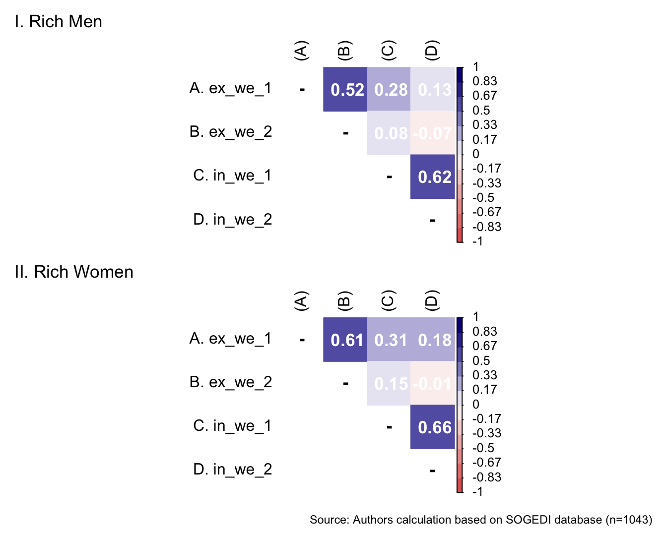
Reliability
mi_variable <- "ex_atri_we"
result2 <- alphas(db_proc, c("ex_we_1", "ex_we_2"), mi_variable)

result2$raw_alpha
[1] 0.7187958result2$new_var_summary Min. 1st Qu. Median Mean 3rd Qu. Max. NA's
1.000 5.000 6.000 5.905 7.000 7.000 2110 mi_variable <- "in_atri_we"
result3 <- alphas(db_proc, c("in_we_1", "in_we_2"), mi_variable)
result3$raw_alpha[1] 0.7803945result3$new_var_summary Min. 1st Qu. Median Mean 3rd Qu. Max. NA's
1.000 4.000 5.000 5.049 6.000 7.000 2110 Confirmatory factor analysis
Mardia’s test for evaluate multivariate normality for each target.
mardia(db_rm[,c("ex_we_1", "ex_we_2", "in_we_1", "in_we_2")],
       na.rm = T, plot=T)
Call: mardia(x = db_rm[, c(“ex_we_1”, “ex_we_2”, “in_we_1”, “in_we_2”)], na.rm = T, plot = T)
Mardia tests of multivariate skew and kurtosis Use describe(x) the to get univariate tests n.obs = 1043 num.vars = 4 b1p = 5.84 skew = 1014.66 with probability <= 0.00000000000000000000000000000000000000000000000000000000000000000000000000000000000000000000000000000000000000000000000000000000000000000000000000000000000000000000000000000000000000000000000000000000029 small sample skew = 1018.75 with probability <= 0.000000000000000000000000000000000000000000000000000000000000000000000000000000000000000000000000000000000000000000000000000000000000000000000000000000000000000000000000000000000000000000000000000000000039 b2p = 35.88 kurtosis = 27.69 with probability <= 0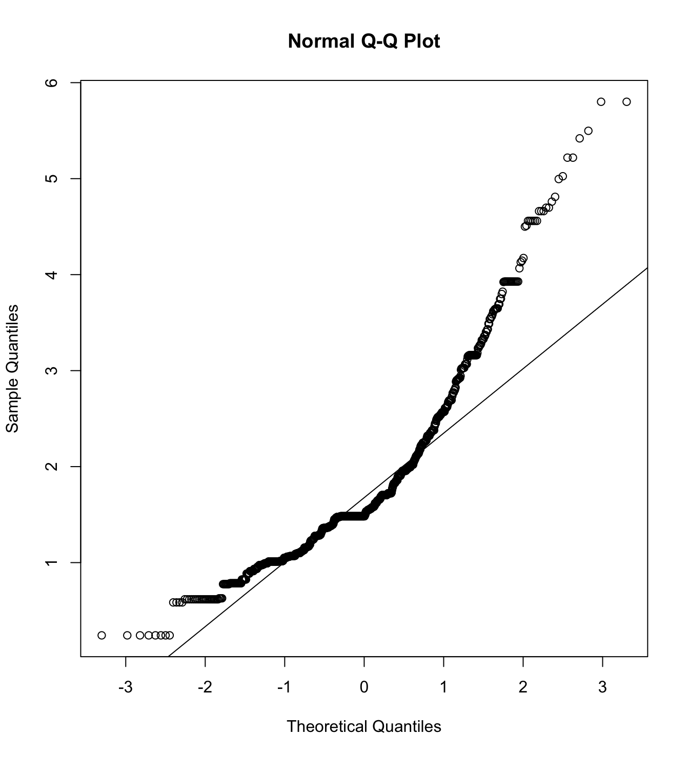
mardia(db_rw[,c("ex_we_1", "ex_we_2", "in_we_1", "in_we_2")],
       na.rm = T, plot=T)
Call: mardia(x = db_rw[, c(“ex_we_1”, “ex_we_2”, “in_we_1”, “in_we_2”)], na.rm = T, plot = T)
Mardia tests of multivariate skew and kurtosis Use describe(x) the to get univariate tests n.obs = 1056 num.vars = 4 b1p = 5.26 skew = 926.15 with probability <= 0.0000000000000000000000000000000000000000000000000000000000000000000000000000000000000000000000000000000000000000000000000000000000000000000000000000000000000000000000000000000000000021 small sample skew = 929.84 with probability <= 0.00000000000000000000000000000000000000000000000000000000000000000000000000000000000000000000000000000000000000000000000000000000000000000000000000000000000000000000000000000000000000035 b2p = 36.67 kurtosis = 29.71 with probability <= 0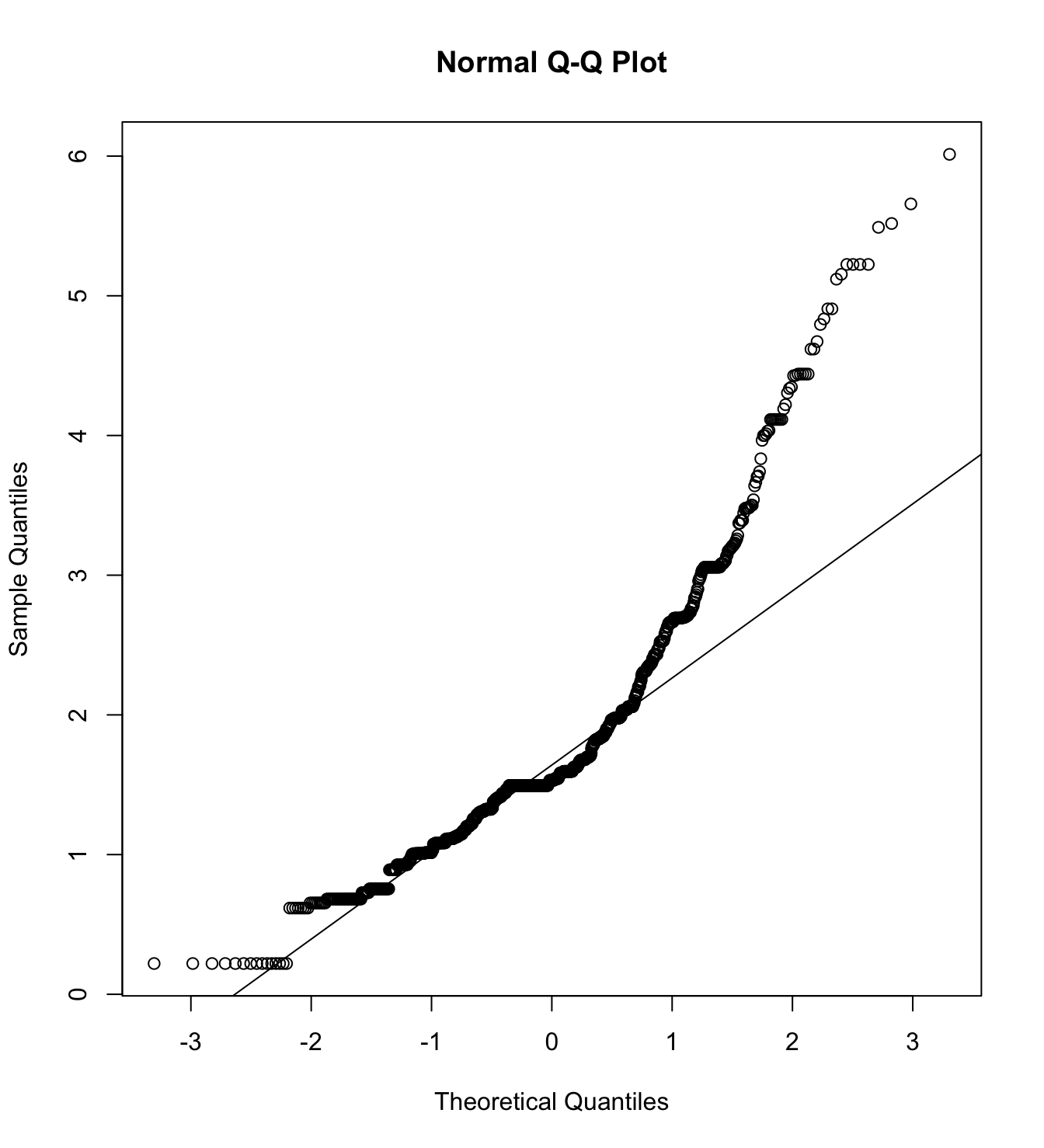
We first specify the factorial structure of the items, then fit models using a robust maximum likelihood estimator for the entire sample as well as for each country individually. The goodnes of fit indicators are shown.
# model
model_cfa <- '
  external_atri_we =~ ex_we_1 + ex_we_2
  internal_atri_we =~ in_we_1 + in_we_2
'

# estimation
# overall
m15_cfa_rm <- cfa(model = model_cfa,
              data = subset(db_proc, target == "Rich.Men"),
              estimator = "MLR",
              ordered = F,
              std.lv = F)

m15_cfa_rw <- cfa(model = model_cfa,
              data = subset(db_proc, target == "Rich.Women"),
              estimator = "MLR",
              ordered = F,
              std.lv = F)

# argentina
m15_cfa_rm_arg <- cfa(model = model_cfa,
                 data = subset(db_proc, group == "1.Rich.Men"),
                 estimator = "MLR",
                 ordered = F,
                 std.lv = F)

m15_cfa_rw_arg <- cfa(model = model_cfa,
                 data = subset(db_proc, group == "1.Rich.Women"),
                 estimator = "MLR",
                 ordered = F,
                 std.lv = F)

# chile
m15_cfa_rm_cl <- cfa(model = model_cfa,
                     data = subset(db_proc, group == "3.Rich.Men"),
                     estimator = "MLR",
                     ordered = F,
                     std.lv = F)


m15_cfa_rw_cl <- cfa(model = model_cfa,
                     data = subset(db_proc, group == "3.Rich.Women"),
                     estimator = "MLR",
                     ordered = F,
                     std.lv = F)

# colombia
m15_cfa_rm_col <- cfa(model = model_cfa,
                     data = subset(db_proc, group == "4.Rich.Men"),
                     estimator = "MLR",
                     ordered = F,
                     std.lv = F)


m15_cfa_rw_col <- cfa(model = model_cfa,
                     data = subset(db_proc, group == "4.Rich.Women"),
                     estimator = "MLR",
                     ordered = F,
                     std.lv = F)


# españa
m15_cfa_rm_esp <- cfa(model = model_cfa,
                     data = subset(db_proc, group == "9.Rich.Men"),
                     estimator = "MLR",
                     ordered = F,
                     std.lv = F)


m15_cfa_rw_esp <- cfa(model = model_cfa,
                     data = subset(db_proc, group == "9.Rich.Women"),
                     estimator = "MLR",
                     ordered = F,
                     std.lv = F)


# mexico
m15_cfa_rm_mex <- cfa(model = model_cfa,
                     data = subset(db_proc, group == "13.Rich.Men"),
                     estimator = "MLR",
                     ordered = F,
                     std.lv = F)


m15_cfa_rw_mex <- cfa(model = model_cfa,
                     data = subset(db_proc, group == "13.Rich.Women"),
                     estimator = "MLR",
                     ordered = F,
                     std.lv = F)
colnames_fit <- c("","Target","$N$","Estimator","$\\chi^2$ (df)","CFI","TLI","RMSEA 90% CI [Lower-Upper]", "SRMR", "AIC")
bind_rows(
cfa_tab_fit(
models = list(m15_cfa_rm, m15_cfa_rm_cl, m15_cfa_rm_col, m15_cfa_rm_esp, m15_cfa_rm_mex),
country_names = c("Overall scores", "Chile", "Colombia", "Spain", "México")
)$sum_fit %>%
mutate(target = "Rich Men")
,
cfa_tab_fit(
models = list(m15_cfa_rw, m15_cfa_rw_arg, m15_cfa_rw_cl, m15_cfa_rw_col, m15_cfa_rw_esp, m15_cfa_rw_mex),
country_names = c("Overall scores", "Argentina", "Chile", "Colombia", "Spain", "México")
)$sum_fit %>%
mutate(target = "Rich Women")
) %>%
select(country, target, everything()) %>%
mutate(country = factor(country, levels = c("Overall scores", "Argentina", "Chile", "Colombia", "Spain", "México"))) %>%
group_by(country) %>%
arrange(country) %>%
mutate(country = if_else(duplicated(country), NA, country)) %>%
kableExtra::kable(
format = "markdown",
digits = 3,
booktabs = TRUE,
col.names = colnames_fit,
caption = NULL
) %>%
kableExtra::kable_styling(
full_width = TRUE,
font_size = 11,
latex_options = "HOLD_position",
bootstrap_options = c("striped", "bordered")
) %>%
kableExtra::collapse_rows(columns = 1)| Target | \(N\) | Estimator | \(\chi^2\) (df) | CFI | TLI | RMSEA 90% CI [Lower-Upper] | SRMR | AIC | |
|---|---|---|---|---|---|---|---|---|---|
| Overall scores | Rich Men | 1043 | ML | 24.221 (1) *** | 0.975 | 0.853 | 0.149 [0.101-0.203] | 0.040 | 14406.862 |
| Rich Women | 1056 | ML | 30.881 (1) *** | 0.976 | 0.853 | 0.168 [0.12-0.222] | 0.035 | 14360.205 | |
| Argentina | Rich Women | 207 | ML | 5.55 (1) * | 0.981 | 0.883 | 0.148 [0.049-0.278] | 0.035 | 2807.519 |
| Chile | Rich Men | 217 | ML | 4.044 (1) * | 0.988 | 0.927 | 0.118 [0.016-0.248] | 0.034 | 2992.819 |
| Rich Women | 223 | ML | 20.83 (1) *** | 0.923 | 0.539 | 0.298 [0.195-0.416] | 0.056 | 3067.145 | |
| Colombia | Rich Men | 206 | ML | 0.143 (1) | 1.000 | 1.029 | 0 [0-0.134] | 0.006 | 2790.397 |
| Rich Women | 199 | ML | 1.171 (1) | 0.999 | 0.994 | 0.029 [0-0.193] | 0.017 | 2672.028 | |
| Spain | Rich Men | 195 | ML | 8.567 (1) ** | 0.969 | 0.814 | 0.197 [0.092-0.327] | 0.066 | 2509.596 |
| Rich Women | 212 | ML | 3.819 (1) . | 0.992 | 0.954 | 0.115 [0-0.247] | 0.024 | 2689.485 | |
| México | Rich Men | 209 | ML | 8.055 (1) ** | 0.958 | 0.746 | 0.184 [0.083-0.31] | 0.050 | 2998.907 |
| Rich Women | 215 | ML | 1.164 (1) | 0.999 | 0.995 | 0.028 [0-0.186] | 0.016 | 3025.332 |
5.6 Block 6. Poverty Implications
5.6.1 Thick skin bias
We reduced the amount of items that the original authors used and silly adapted to our context of study (Cheek & Shafir, 2024). We did not find any information regarding factorial analyses so we selected the items that were more likely to be applied to low-SES groups in our context.
Descriptive analysis
describe_kable(db_proc, c("sk_1", "sk_2", "sk_3"))| vars | n | mean | sd | median | trimmed | mad | min | max | range | skew | kurtosis | se | |
|---|---|---|---|---|---|---|---|---|---|---|---|---|---|
| sk_1 | 1 | 4209 | 5.292 | 1.773 | 6 | 5.533 | 1.483 | 1 | 7 | 6 | -0.804 | -0.305 | 0.027 |
| sk_2 | 2 | 4209 | 5.540 | 1.748 | 6 | 5.828 | 1.483 | 1 | 7 | 6 | -1.058 | 0.156 | 0.027 |
| sk_3 | 3 | 4209 | 5.442 | 1.787 | 6 | 5.725 | 1.483 | 1 | 7 | 6 | -0.975 | -0.049 | 0.028 |
wrap_elements(
    ~corrplot::corrplot(
      fit_correlations(db_proc, c("sk_1", "sk_2", "sk_3")),
      method = "color",
      type = "upper",
      col = colorRampPalette(c("#E16462", "white", "#0D0887"))(12),
      tl.pos = "lt",
      tl.col = "black",
      addrect = 2,
      rect.col = "black",
      addCoef.col = "white",
      cl.cex = 0.8,
      cl.align.text = 'l',
      number.cex = 1.1,
      na.label = "-",
      bg = "white"
    )
  ) +
    plot_annotation(
      caption = paste0(
        "Source: Authors calculation based on SOGEDI database"
      )
    )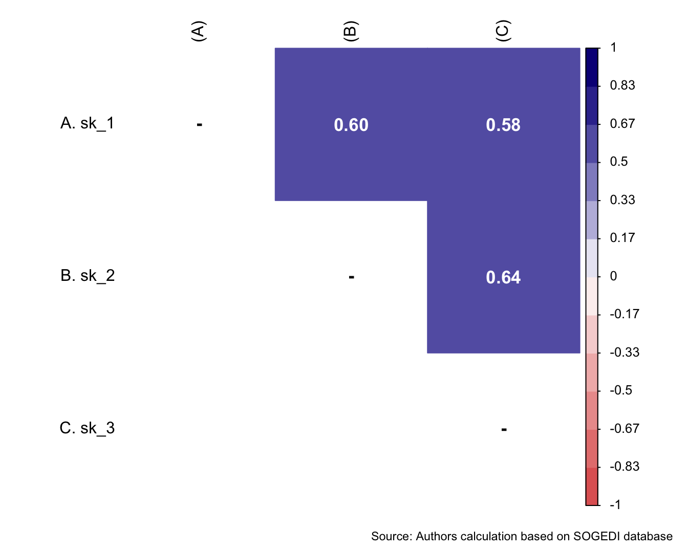
Reliability
mi_variable <- "skin"
result2 <- alphas(db_proc, c("sk_1", "sk_2", "sk_3"), mi_variable)

result2$raw_alpha
[1] 0.8232648result2$new_var_summary Min. 1st Qu. Median Mean 3rd Qu. Max.
1.000 4.333 5.667 5.424 7.000 7.000 Confirmatory factor analysis
Mardia’s test for evaluate multivariate normality.
mardia(db_proc[,c("sk_1", "sk_2", "sk_3")],
       na.rm = T, plot=T)
Call: mardia(x = db_proc[, c(“sk_1”, “sk_2”, “sk_3”)], na.rm = T, plot = T)
Mardia tests of multivariate skew and kurtosis Use describe(x) the to get univariate tests n.obs = 4209 num.vars = 3 b1p = 3.12 skew = 2188.55 with probability <= 0 small sample skew = 2190.89 with probability <= 0 b2p = 24.77 kurtosis = 57.84 with probability <= 0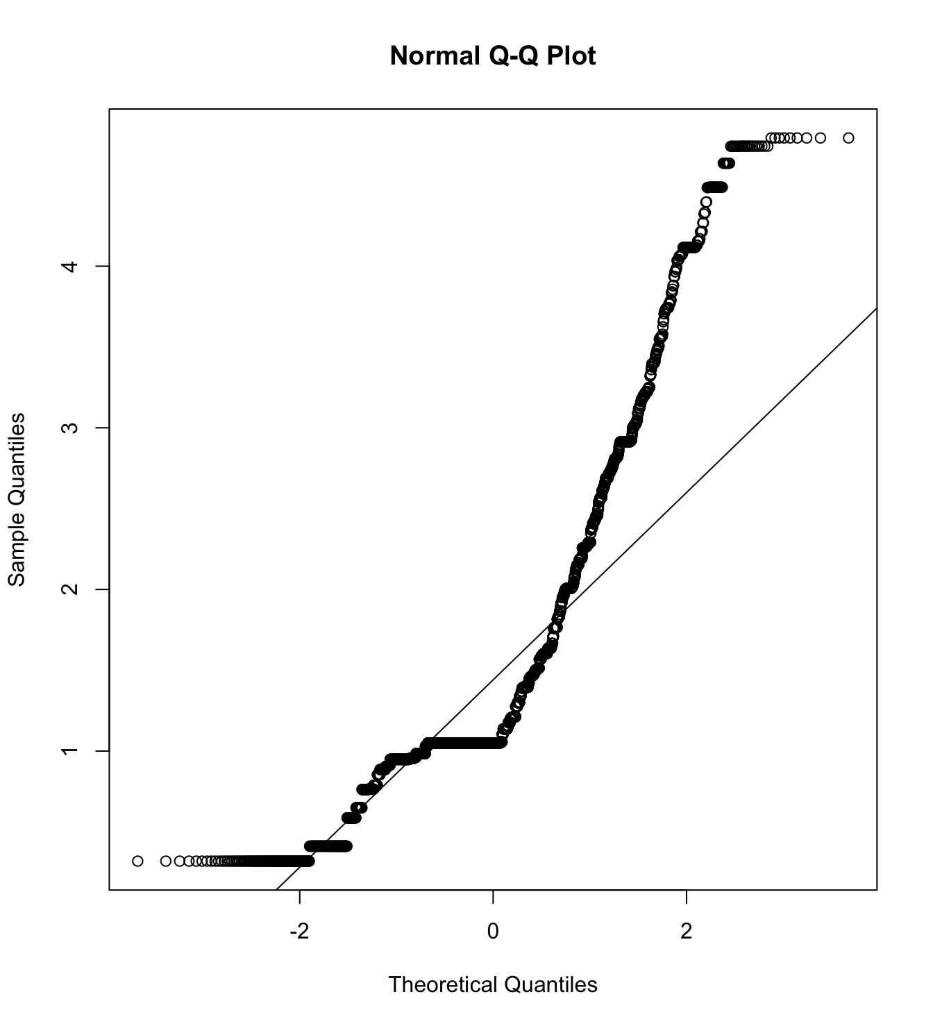
We first specify the factorial structure of the items, then fit models using a robust maximum likelihood estimator for the entire sample as well as for each country individually. The goodnes of fit indicators are shown.
# model
model_cfa <- '
  skin_bias =~ sk_1 + sk_2 + sk_3
'

# estimation
# overall
m16_cfa <- cfa(model = model_cfa,
              data = db_proc,
              estimator = "MLR",
              ordered = F,
              std.lv = F)

# argentina
m16_cfa_arg <- cfa(model = model_cfa,
                 data = subset(db_proc, country_residence_recoded == 1),
                 estimator = "MLR",
                 ordered = F,
                 std.lv = F)

# chile
m16_cfa_cl <- cfa(model = model_cfa,
                     data = subset(db_proc, country_residence_recoded == 3),
                     estimator = "MLR",
                     ordered = F,
                     std.lv = F)


# colombia
m16_cfa_col <- cfa(model = model_cfa,
                     data = subset(db_proc, country_residence_recoded == 4),
                     estimator = "MLR",
                     ordered = F,
                     std.lv = F)


# españa
m16_cfa_esp <- cfa(model = model_cfa,
                     data = subset(db_proc, country_residence_recoded == 9),
                     estimator = "MLR",
                     ordered = F,
                     std.lv = F)


# mexico
m16_cfa_mex <- cfa(model = model_cfa,
                     data = subset(db_proc, country_residence_recoded == 13),
                     estimator = "MLR",
                     ordered = F,
std.lv = F) cfa_tab_fit(
models = list(m16_cfa, m16_cfa_arg, m16_cfa_cl, m16_cfa_col, m16_cfa_esp, m16_cfa_mex),
country_names = c("Overall scores", "Argentina", "Chile", "Colombia", "Spain", "México")
)$fit_table| \(N\) | Estimator | \(\chi^2\) (df) | CFI | TLI | RMSEA 90% CI [Lower-Upper] | SRMR | AIC | |
|---|---|---|---|---|---|---|---|---|
| Overall scores | 4209 | ML | 0 (0) | 1 | 1 | 0 [0-0] | 0 | 45672.145 |
| Argentina | 807 | ML | 0 (0) | 1 | 1 | 0 [0-0] | 0 | 8564.323 |
| Chile | 883 | ML | 0 (0) | 1 | 1 | 0 [0-0] | 0 | 9455.343 |
| Colombia | 833 | ML | 0 (0) | 1 | 1 | 0 [0-0] | 0 | 9437.460 |
| Spain | 835 | ML | 0 (0) | 1 | 1 | 0 [0-0] | 0 | 8238.133 |
| México | 846 | ML | 0 (0) | 1 | 1 | 0 [0-0] | 0 | 9547.576 |
5.6.2 Deservingness
Items adapted (own translation) from Meleuman, Roosma & Abts (2020). These items are uniquely presented for participants in the poverty condition.
Descriptive analysis
db_proc$carin_control_2_r <- sjmisc::rec(db_proc$carin_control_2,rec = "rev")
db_pm$carin_control_2_r <- sjmisc::rec(db_pm$carin_control_2,rec = "rev")
db_pw$carin_control_2_r <- sjmisc::rec(db_pw$carin_control_2,rec = "rev")

bind_rows(
psych::describe(db_pm[,c("carin_control_1","carin_control_2_r","carin_attitude_1","carin_attitude_2","carin_reciprocity_1","carin_reciprocity_2","carin_identity_1","carin_identity_2","carin_need_1","carin_need_2")]) %>%
    as_tibble() %>%
    mutate(target = "Poor Men")
,
psych::describe(db_pw[,c("carin_control_1","carin_control_2_r","carin_attitude_1","carin_attitude_2","carin_reciprocity_1","carin_reciprocity_2","carin_identity_1","carin_identity_2","carin_need_1","carin_need_2")]) %>%
    as_tibble() %>%
    mutate(target = "Poor Women")
) %>%
  mutate(vars = case_when(vars %in% c(1:2) ~ paste0("carin_control_", vars),
                          vars %in% c(3:4) ~ paste0("carin_attitude_", vars),
                          vars %in% c(5:6) ~ paste0("carin_reciprocity_", vars),
                          vars %in% c(7:8) ~ paste0("carin_identity_", vars),
                          vars %in% c(9:10) ~ paste0("carin_need_", vars))) %>%
  select(target, everything()) %>%
  group_by(target) %>%
  mutate(target = if_else(duplicated(target), NA, target)) %>%
kableExtra::kable(format = "markdown", digits = 3)| target | vars | n | mean | sd | median | trimmed | mad | min | max | range | skew | kurtosis | se |
|---|---|---|---|---|---|---|---|---|---|---|---|---|---|
| Poor Men | carin_control_1 | 1058 | 3.907 | 1.916 | 4 | 3.884 | 1.483 | 1 | 7 | 6 | 0.105 | -0.990 | 0.059 |
| carin_control_2 | 1058 | 4.883 | 1.860 | 5 | 5.067 | 2.965 | 1 | 7 | 6 | -0.503 | -0.744 | 0.057 | |
| carin_attitude_3 | 1058 | 4.466 | 1.988 | 4 | 4.581 | 2.965 | 1 | 7 | 6 | -0.256 | -1.052 | 0.061 | |
| carin_attitude_4 | 1058 | 2.891 | 1.871 | 2 | 2.654 | 1.483 | 1 | 7 | 6 | 0.696 | -0.574 | 0.058 | |
| carin_reciprocity_5 | 1058 | 3.504 | 1.997 | 4 | 3.381 | 2.965 | 1 | 7 | 6 | 0.232 | -1.095 | 0.061 | |
| carin_reciprocity_6 | 1058 | 4.486 | 2.111 | 5 | 4.606 | 2.965 | 1 | 7 | 6 | -0.386 | -1.112 | 0.065 | |
| carin_identity_7 | 1058 | 3.378 | 2.172 | 3 | 3.224 | 2.965 | 1 | 7 | 6 | 0.353 | -1.251 | 0.067 | |
| carin_identity_8 | 1058 | 4.678 | 2.223 | 5 | 4.846 | 2.965 | 1 | 7 | 6 | -0.464 | -1.209 | 0.068 | |
| carin_need_9 | 1058 | 3.571 | 2.186 | 4 | 3.465 | 2.965 | 1 | 7 | 6 | 0.232 | -1.334 | 0.067 | |
| carin_need_10 | 1058 | 3.967 | 2.112 | 4 | 3.959 | 2.965 | 1 | 7 | 6 | -0.029 | -1.290 | 0.065 | |
| Poor Women | carin_control_1 | 1052 | 4.085 | 1.941 | 4 | 4.106 | 2.965 | 1 | 7 | 6 | -0.017 | -1.053 | 0.060 |
| carin_control_2 | 1052 | 5.585 | 1.659 | 6 | 5.846 | 1.483 | 1 | 7 | 6 | -1.012 | 0.155 | 0.051 | |
| carin_attitude_3 | 1052 | 4.087 | 2.036 | 4 | 4.109 | 2.965 | 1 | 7 | 6 | -0.106 | -1.133 | 0.063 | |
| carin_attitude_4 | 1052 | 2.656 | 1.838 | 2 | 2.380 | 1.483 | 1 | 7 | 6 | 0.868 | -0.311 | 0.057 | |
| carin_reciprocity_5 | 1052 | 3.104 | 1.951 | 3 | 2.904 | 2.965 | 1 | 7 | 6 | 0.495 | -0.909 | 0.060 | |
| carin_reciprocity_6 | 1052 | 3.954 | 2.158 | 4 | 3.943 | 2.965 | 1 | 7 | 6 | -0.052 | -1.340 | 0.067 | |
| carin_identity_7 | 1052 | 2.950 | 2.069 | 2 | 2.692 | 1.483 | 1 | 7 | 6 | 0.662 | -0.890 | 0.064 | |
| carin_identity_8 | 1052 | 4.414 | 2.289 | 5 | 4.518 | 2.965 | 1 | 7 | 6 | -0.284 | -1.408 | 0.071 | |
| carin_need_9 | 1052 | 3.471 | 2.217 | 3 | 3.340 | 2.965 | 1 | 7 | 6 | 0.312 | -1.313 | 0.068 | |
| carin_need_10 | 1052 | 3.794 | 2.144 | 4 | 3.742 | 2.965 | 1 | 7 | 6 | 0.096 | -1.309 | 0.066 |
p1 <- wrap_elements(
    ~corrplot::corrplot(
      fit_correlations_pairwise(db_pm, c("carin_control_1","carin_control_2_r","carin_attitude_1","carin_attitude_2","carin_reciprocity_1","carin_reciprocity_2","carin_identity_1","carin_identity_2","carin_need_1","carin_need_2")),
      method = "color",
      type = "upper",
      col = colorRampPalette(c("#E16462", "white", "#0D0887"))(12),
      tl.pos = "lt",
      tl.col = "black",
      addrect = 2,
      rect.col = "black",
      addCoef.col = "white",
      cl.cex = 0.8,
      cl.align.text = 'l',
      number.cex = 1.1,
      na.label = "-",
      bg = "white"
    )
  ) + labs(title = "I. Poor Men")


p2 <- wrap_elements(
    ~corrplot::corrplot(
      fit_correlations_pairwise(db_pw, c("carin_control_1","carin_control_2_r","carin_attitude_1","carin_attitude_2","carin_reciprocity_1","carin_reciprocity_2","carin_identity_1","carin_identity_2","carin_need_1","carin_need_2")),
      method = "color",
      type = "upper",
      col = colorRampPalette(c("#E16462", "white", "#0D0887"))(12),
      tl.pos = "lt",
      tl.col = "black",
      addrect = 2,
      rect.col = "black",
      addCoef.col = "white",
      cl.cex = 0.8,
      cl.align.text = 'l',
      number.cex = 1.1,
      na.label = "-",
      bg = "white"
    )
  ) + labs(title = "II. Poor Women")


p1/p2 +
    plot_annotation(
      caption = paste0(
        "Source: Authors calculation based on SOGEDI database"
      )
    )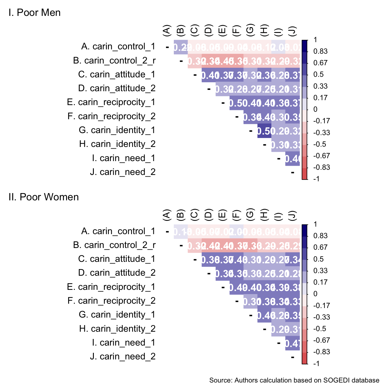
Reliability
mi_variable <- "carin_control"
result2 <- alphas(db_proc, c("carin_control_1","carin_control_2_r"), mi_variable)

result2$raw_alpha
[1] 0.3047283result2$new_var_summary Min. 1st Qu. Median Mean 3rd Qu. Max. NA's
1.000 4.000 4.500 4.614 5.500 7.000 2099 mi_variable <- "carin_attitude"
result2 <- alphas(db_proc, c("carin_attitude_1","carin_attitude_2"), mi_variable)
result2$raw_alpha[1] 0.5674176result2$new_var_summary Min. 1st Qu. Median Mean 3rd Qu. Max. NA's
1.000 2.500 3.500 3.526 4.500 7.000 2099 mi_variable <- "carin_reciprocity"
result2 <- alphas(db_proc, c("carin_reciprocity_1","carin_reciprocity_2"), mi_variable)
result2$raw_alpha[1] 0.6654127result2$new_var_summary Min. 1st Qu. Median Mean 3rd Qu. Max. NA's
1.000 2.500 4.000 3.763 5.000 7.000 2099 mi_variable <- "carin_identity"
result2 <- alphas(db_proc, c("carin_identity_1","carin_identity_2"), mi_variable)
result2$raw_alpha[1] 0.6494677result2$new_var_summary Min. 1st Qu. Median Mean 3rd Qu. Max. NA's
1.000 2.500 4.000 3.856 5.500 7.000 2099 mi_variable <- "carin_need"
result2 <- alphas(db_proc, c("carin_need_1","carin_need_2"), mi_variable)
result2$raw_alpha[1] 0.6357058result2$new_var_summary Min. 1st Qu. Median Mean 3rd Qu. Max. NA's
1.000 2.000 4.000 3.701 5.000 7.000 2099 Confirmatory factor analysis
Mardia’s test for evaluate multivariate normality.
mardia(db_pm[,c("carin_control_1","carin_control_2_r","carin_attitude_1","carin_attitude_2","carin_reciprocity_1","carin_reciprocity_2","carin_identity_1","carin_identity_2","carin_need_1","carin_need_2")],
       na.rm = T, plot=T)
Call: mardia(x = db_pm[, c(“carin_control_1”, “carin_control_2_r”, “carin_attitude_1”, “carin_attitude_2”, “carin_reciprocity_1”, “carin_reciprocity_2”, “carin_identity_1”, “carin_identity_2”, “carin_need_1”, “carin_need_2”)], na.rm = T, plot = T)
Mardia tests of multivariate skew and kurtosis Use describe(x) the to get univariate tests n.obs = 1058 num.vars = 10 b1p = 4.9 skew = 864.84 with probability <= 0.00000000000000000000000000000000000000000000000000000000000000000000000000003 small sample skew = 867.74 with probability <= 0.00000000000000000000000000000000000000000000000000000000000000000000000000001 b2p = 134.56 kurtosis = 15.28 with probability <= 0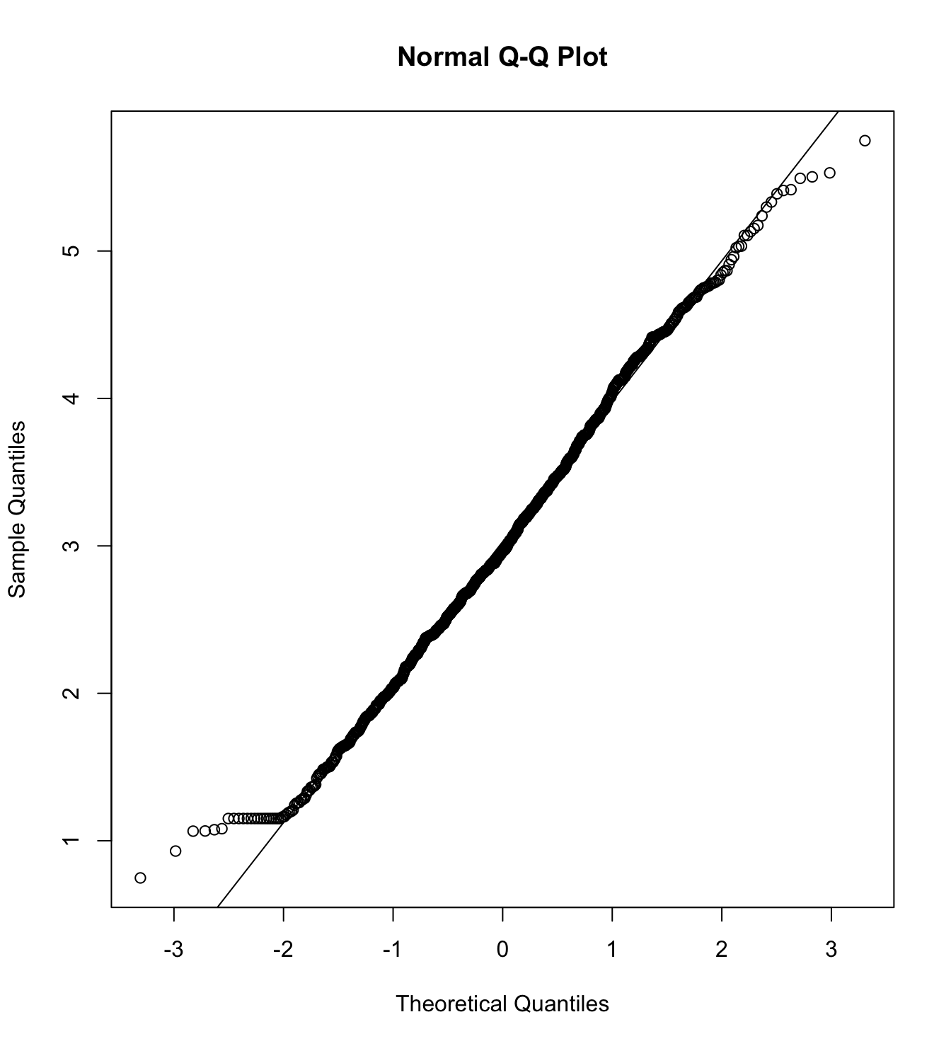
mardia(db_pw[,c("carin_control_1","carin_control_2_r","carin_attitude_1","carin_attitude_2","carin_reciprocity_1","carin_reciprocity_2","carin_identity_1","carin_identity_2","carin_need_1","carin_need_2")],
       na.rm = T, plot=T)
Call: mardia(x = db_pw[, c(“carin_control_1”, “carin_control_2_r”, “carin_attitude_1”, “carin_attitude_2”, “carin_reciprocity_1”, “carin_reciprocity_2”, “carin_identity_1”, “carin_identity_2”, “carin_need_1”, “carin_need_2”)], na.rm = T, plot = T)
Mardia tests of multivariate skew and kurtosis Use describe(x) the to get univariate tests n.obs = 1052 num.vars = 10 b1p = 6.14 skew = 1076.46 with probability <= 0.000000000000000000000000000000000000000000000000000000000000000000000000000000000000000000000000000000000000000073 small sample skew = 1080.09 with probability <= 0.000000000000000000000000000000000000000000000000000000000000000000000000000000000000000000000000000000000000000017 b2p = 137.99 kurtosis = 18.83 with probability <= 0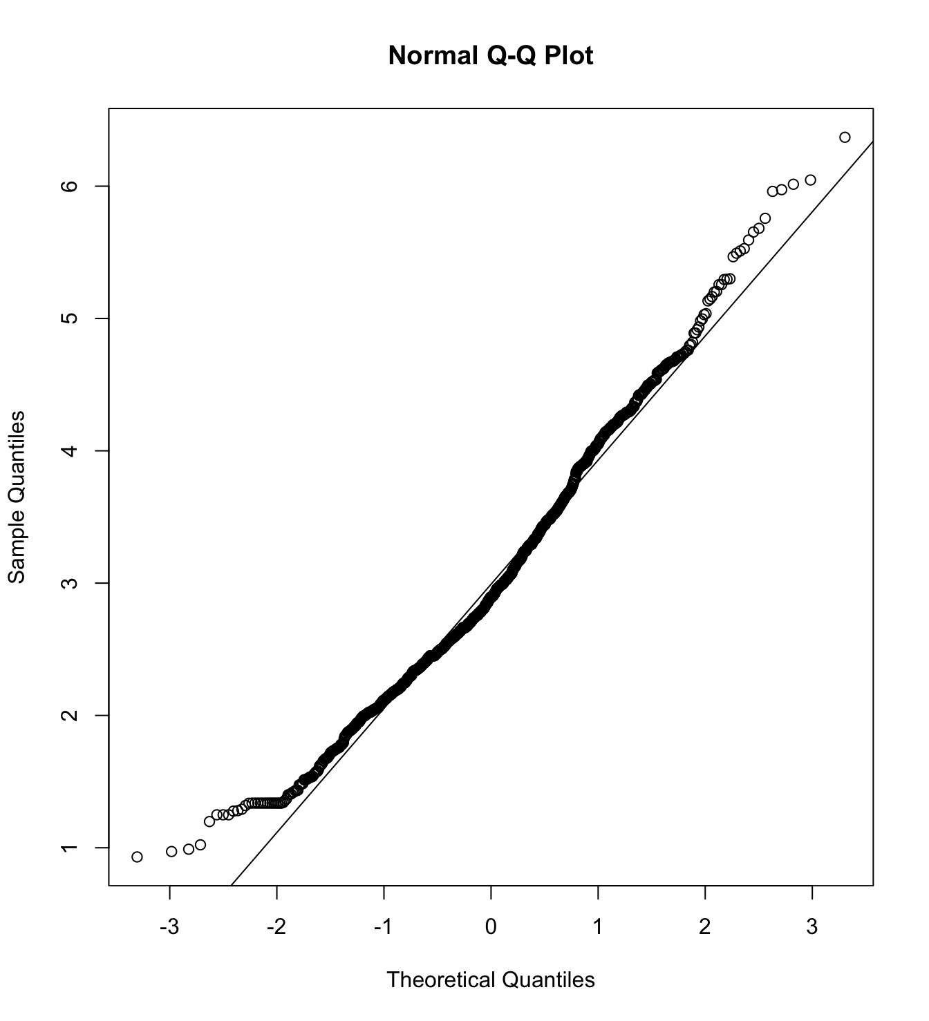
We first specify the factorial structure of the items, then fit models using a robust maximum likelihood estimator for the entire sample as well as for each country individually. The goodnes of fit indicators are shown.
# model
model_cfa <- '
  control =~ carin_control_1 + carin_control_2_r
  attitude =~ carin_attitude_1 + carin_attitude_2
  reciprocity =~ carin_reciprocity_1 + carin_reciprocity_2
  identity =~ carin_identity_1 + carin_identity_2
  need =~ carin_need_1 + carin_need_2
'

# estimation
# overall
m17_cfa_pm <- cfa(model = model_cfa,
              data = subset(db_proc, target == "Poor.Men"),
              estimator = "MLR",
              ordered = F,
              std.lv = F)

m17_cfa_pw <- cfa(model = model_cfa,
              data = subset(db_proc, target == "Poor.Women"),
              estimator = "MLR",
              ordered = F,
              std.lv = F)

# argentina
m17_cfa_pm_arg <- cfa(model = model_cfa,
                 data = subset(db_proc, group == "1.Poor.Men"),
                 estimator = "MLR",
                 ordered = F,
                 std.lv = F)

m17_cfa_pw_arg <- cfa(model = model_cfa,
                 data = subset(db_proc, group == "1.Poor.Women"),
                 estimator = "MLR",
                 ordered = F,
                 std.lv = F)

# chile
m17_cfa_pm_cl <- cfa(model = model_cfa,
                     data = subset(db_proc, group == "3.Poor.Men"),
                     estimator = "MLR",
                     ordered = F,
                     std.lv = F)


m17_cfa_pw_cl <- cfa(model = model_cfa,
                     data = subset(db_proc, group == "3.Poor.Women"),
                     estimator = "MLR",
                     ordered = F,
                     std.lv = F)

# colombia
m17_cfa_pm_col <- cfa(model = model_cfa,
                     data = subset(db_proc, group == "4.Poor.Men"),
                     estimator = "MLR",
                     ordered = F,
                     std.lv = F)


m17_cfa_pw_col <- cfa(model = model_cfa,
                     data = subset(db_proc, group == "4.Poor.Women"),
                     estimator = "MLR",
                     ordered = F,
                     std.lv = F)


# españa
m17_cfa_pm_esp <- cfa(model = model_cfa,
                     data = subset(db_proc, group == "9.Poor.Men"),
                     estimator = "MLR",
                     ordered = F,
                     std.lv = F)


m17_cfa_pw_esp <- cfa(model = model_cfa,
                     data = subset(db_proc, group == "9.Poor.Women"),
                     estimator = "MLR",
                     ordered = F,
                     std.lv = F)


# mexico
m17_cfa_pm_mex <- cfa(model = model_cfa,
                     data = subset(db_proc, group == "13.Poor.Men"),
                     estimator = "MLR",
                     ordered = F,
                     std.lv = F)


m17_cfa_pw_mex <- cfa(model = model_cfa,
                     data = subset(db_proc, group == "13.Poor.Women"),
                     estimator = "MLR",
                     ordered = F,
                     std.lv = F)
colnames_fit <- c("","Target","$N$","Estimator","$\\chi^2$ (df)","CFI","TLI","RMSEA 90% CI [Lower-Upper]", "SRMR", "AIC")
bind_rows(
cfa_tab_fit(
models = list(m17_cfa_pm, m17_cfa_pm_arg, m17_cfa_pm_esp, m17_cfa_pm_mex),
country_names = c("Overall scores", "Argentina", "Spain", "México")
)$sum_fit %>%
mutate(target = "Poor Men")
,
cfa_tab_fit(
models = list(m17_cfa_pw, m17_cfa_pw_arg, m17_cfa_pw_cl, m17_cfa_pw_col, m17_cfa_pw_esp, m17_cfa_pw_mex),
country_names = c("Overall scores", "Argentina", "Chile", "Colombia", "Spain", "México")
)$sum_fit %>%
mutate(target = "Poor Women")
) %>%
select(country, target, everything()) %>%
mutate(country = factor(country, levels = c("Overall scores", "Argentina", "Chile", "Colombia", "Spain", "México"))) %>%
group_by(country) %>%
arrange(country) %>%
mutate(country = if_else(duplicated(country), NA, country)) %>%
kableExtra::kable(
format = "markdown",
digits = 3,
booktabs = TRUE,
col.names = colnames_fit,
caption = NULL
) %>%
kableExtra::kable_styling(
full_width = TRUE,
font_size = 11,
latex_options = "HOLD_position",
bootstrap_options = c("striped", "bordered")
) %>%
kableExtra::collapse_rows(columns = 1)| Target | \(N\) | Estimator | \(\chi^2\) (df) | CFI | TLI | RMSEA 90% CI [Lower-Upper] | SRMR | AIC | |
|---|---|---|---|---|---|---|---|---|---|
| Overall scores | Poor Men | 1058 | ML | 61.943 (25) *** | 0.985 | 0.974 | 0.037 [0.026-0.049] | 0.023 | 42659.995 |
| Poor Women | 1052 | ML | 87.901 (25) *** | 0.974 | 0.953 | 0.049 [0.038-0.06] | 0.026 | 42347.411 | |
| Argentina | Poor Men | 219 | ML | 32.865 (25) | 0.985 | 0.972 | 0.038 [0-0.07] | 0.034 | 8867.883 |
| Poor Women | 215 | ML | 49.747 (25) ** | 0.960 | 0.929 | 0.068 [0.04-0.095] | 0.046 | 8541.143 | |
| Chile | Poor Women | 205 | ML | 48.715 (25) ** | 0.944 | 0.900 | 0.068 [0.039-0.096] | 0.046 | 8430.931 |
| Colombia | Poor Women | 205 | ML | 39.816 (25) * | 0.955 | 0.919 | 0.054 [0.017-0.084] | 0.050 | 8262.347 |
| Spain | Poor Men | 213 | ML | 43.057 (25) * | 0.980 | 0.964 | 0.058 [0.026-0.087] | 0.029 | 8035.667 |
| Poor Women | 211 | ML | 24 (25) | 1.000 | 1.002 | 0 [0-0.053] | 0.025 | 7891.841 | |
| México | Poor Men | 197 | ML | 42.347 (25) * | 0.962 | 0.931 | 0.059 [0.025-0.089] | 0.046 | 8045.836 |
| Poor Women | 216 | ML | 43.106 (25) * | 0.953 | 0.915 | 0.058 [0.026-0.086] | 0.043 | 8848.649 |
5.7 Block 7. Dehumanization
5.7.1 Blatant dehumanization
These items comes from the work of Kteily et al. (2015).
Descriptive analysis
describe_kable(db_proc, c("asc_pw", "asc_pm", "asc_rw", "asc_rm"))| vars | n | mean | sd | median | trimmed | mad | min | max | range | skew | kurtosis | se | |
|---|---|---|---|---|---|---|---|---|---|---|---|---|---|
| asc_pw | 1 | 4209 | 53.148 | 21.871 | 51 | 52.536 | 20.756 | 0 | 100 | 100 | 0.208 | -0.222 | 0.337 |
| asc_pm | 2 | 4209 | 51.533 | 21.893 | 50 | 50.868 | 20.756 | 0 | 100 | 100 | 0.252 | -0.219 | 0.337 |
| asc_rw | 3 | 4209 | 66.552 | 21.785 | 70 | 67.838 | 23.722 | 0 | 100 | 100 | -0.535 | 0.021 | 0.336 |
| asc_rm | 4 | 4209 | 67.434 | 21.854 | 70 | 68.893 | 23.722 | 0 | 100 | 100 | -0.616 | 0.162 | 0.337 |
wrap_elements(
    ~corrplot::corrplot(
      fit_correlations(db_proc, c("asc_pw", "asc_pm", "asc_rw", "asc_rm")),
      method = "color",
      type = "upper",
      col = colorRampPalette(c("#E16462", "white", "#0D0887"))(12),
      tl.pos = "lt",
      tl.col = "black",
      addrect = 2,
      rect.col = "black",
      addCoef.col = "white",
      cl.cex = 0.8,
      cl.align.text = 'l',
      number.cex = 1.1,
      na.label = "-",
      bg = "white"
    )
  ) +
    plot_annotation(
      caption = paste0(
        "Source: Authors calculation based on SOGEDI database"
      )
    )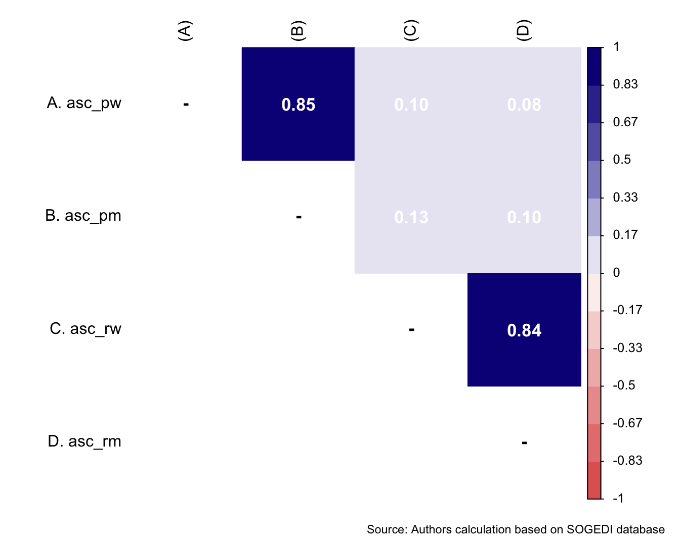
5.8 Block 8. Sexuality
5.8.1 Perceived promiscuity of women
Items taken from Spencer’s work (2016), we changed the response format to fit the survey.
Descriptive analysis
describe_kable(db_proc, c("pro_pw", "pro_rw"))| vars | n | mean | sd | median | trimmed | mad | min | max | range | skew | kurtosis | se | |
|---|---|---|---|---|---|---|---|---|---|---|---|---|---|
| pro_pw | 1 | 4209 | 3.854 | 1.674 | 4 | 3.846 | 1.483 | 1 | 7 | 6 | -0.055 | -0.577 | 0.026 |
| pro_rw | 2 | 4209 | 4.423 | 1.586 | 4 | 4.478 | 1.483 | 1 | 7 | 6 | -0.258 | -0.333 | 0.024 |
wrap_elements(
    ~corrplot::corrplot(
      fit_correlations(db_proc, c("pro_pw", "pro_rw")),
      method = "color",
      type = "upper",
      col = colorRampPalette(c("#E16462", "white", "#0D0887"))(12),
      tl.pos = "lt",
      tl.col = "black",
      addrect = 2,
      rect.col = "black",
      addCoef.col = "white",
      cl.cex = 0.8,
      cl.align.text = 'l',
      number.cex = 1.1,
      na.label = "-",
      bg = "white"
    )
  ) +
    plot_annotation(
      caption = paste0(
        "Source: Authors calculation based on SOGEDI database"
      )
    )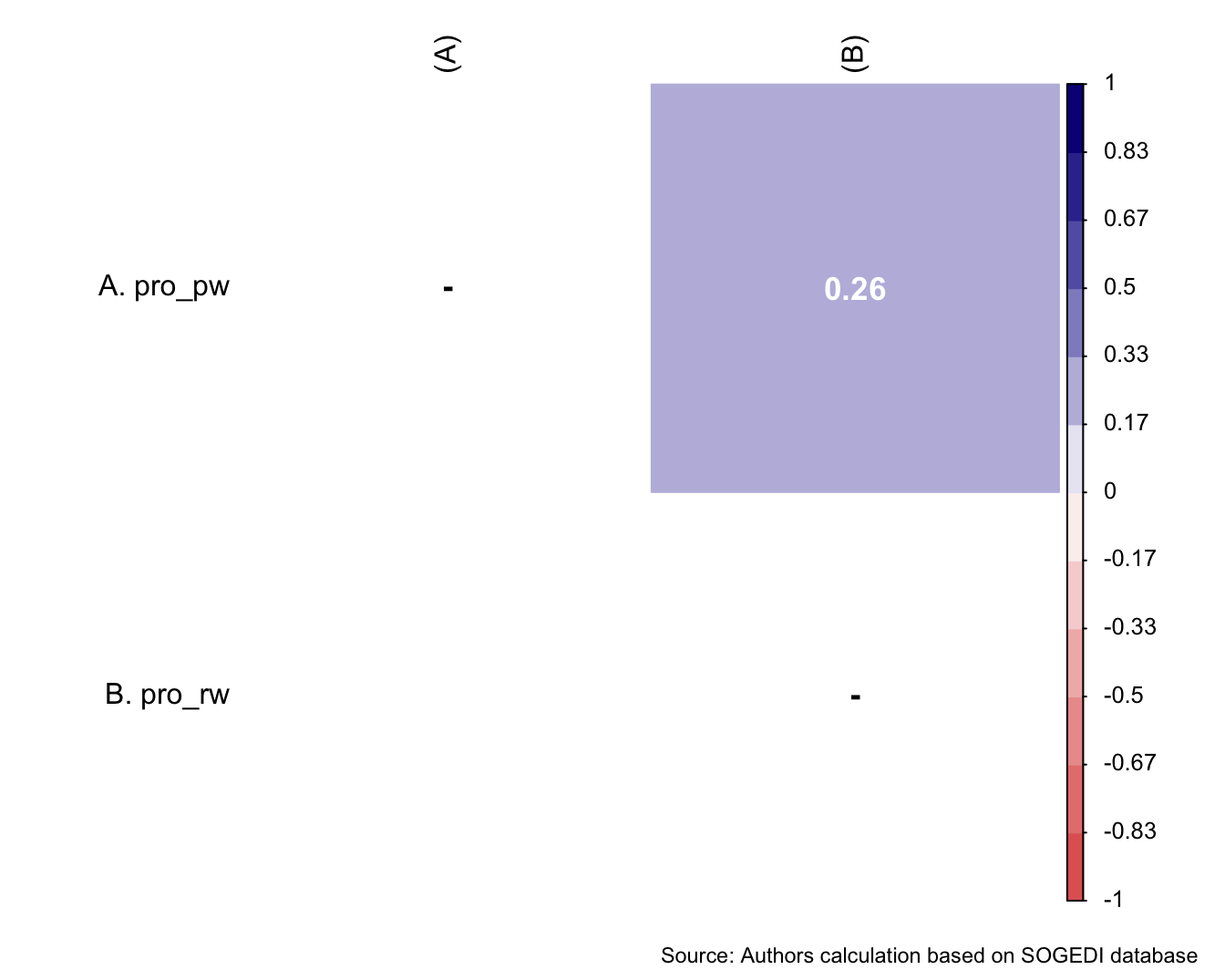
Reliability
5.8.2 Risk sexual behavior of women
In the literature, there are scales to measure this, but they are almost always from a personal perspective (evaluating the risk one takes). We used the scale provided in Raiford et al. (2014) paper to create this single item in order not to lengthen the scale too much.
Descriptive analysis
describe_kable(db_proc, c("ris_pw", "ris_rw"))| vars | n | mean | sd | median | trimmed | mad | min | max | range | skew | kurtosis | se | |
|---|---|---|---|---|---|---|---|---|---|---|---|---|---|
| ris_pw | 1 | 4209 | 5.042 | 1.590 | 5 | 5.189 | 1.483 | 1 | 7 | 6 | -0.577 | -0.208 | 0.025 |
| ris_rw | 2 | 4209 | 4.034 | 1.767 | 4 | 4.042 | 1.483 | 1 | 7 | 6 | -0.001 | -0.802 | 0.027 |
wrap_elements(
    ~corrplot::corrplot(
      fit_correlations(db_proc, c("ris_pw", "ris_rw")),
      method = "color",
      type = "upper",
      col = colorRampPalette(c("#E16462", "white", "#0D0887"))(12),
      tl.pos = "lt",
      tl.col = "black",
      addrect = 2,
      rect.col = "black",
      addCoef.col = "white",
      cl.cex = 0.8,
      cl.align.text = 'l',
      number.cex = 1.1,
      na.label = "-",
      bg = "white"
    )
  ) +
    plot_annotation(
      caption = paste0(
        "Source: Authors calculation based on SOGEDI database"
      )
    )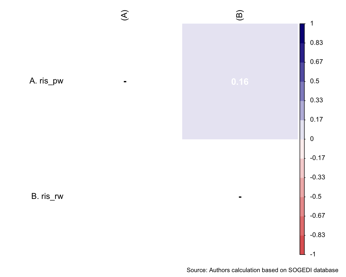
Reliability
5.8.3 Unplanned pregnancy of women
We have created this item, but we believe it could be interesting to explore the idea that poor women have children to take advantage of social assistance. ##### Descriptive analysis
describe_kable(db_proc, c("pre_pw", "pre_rw"))| vars | n | mean | sd | median | trimmed | mad | min | max | range | skew | kurtosis | se | |
|---|---|---|---|---|---|---|---|---|---|---|---|---|---|
| pre_pw | 1 | 4209 | 5.590 | 1.387 | 6 | 5.754 | 1.483 | 1 | 7 | 6 | -0.887 | 0.404 | 0.021 |
| pre_rw | 2 | 4209 | 3.065 | 1.665 | 3 | 2.913 | 1.483 | 1 | 7 | 6 | 0.563 | -0.323 | 0.026 |
wrap_elements(
~corrplot::corrplot(
fit_correlations(db_proc, c("pre_pw", "pre_rw")),
method = "color",
type = "upper",
col = colorRampPalette(c("#E16462", "white", "#0D0887"))(12),
tl.pos = "lt",
tl.col = "black",
addrect = 2,
rect.col = "black",
addCoef.col = "white",
cl.cex = 0.8,
cl.align.text = 'l',
number.cex = 1.1,
na.label = "-",
bg = "white"
)
) +
plot_annotation(
caption = paste0(
"Source: Authors calculation based on SOGEDI database"
)
)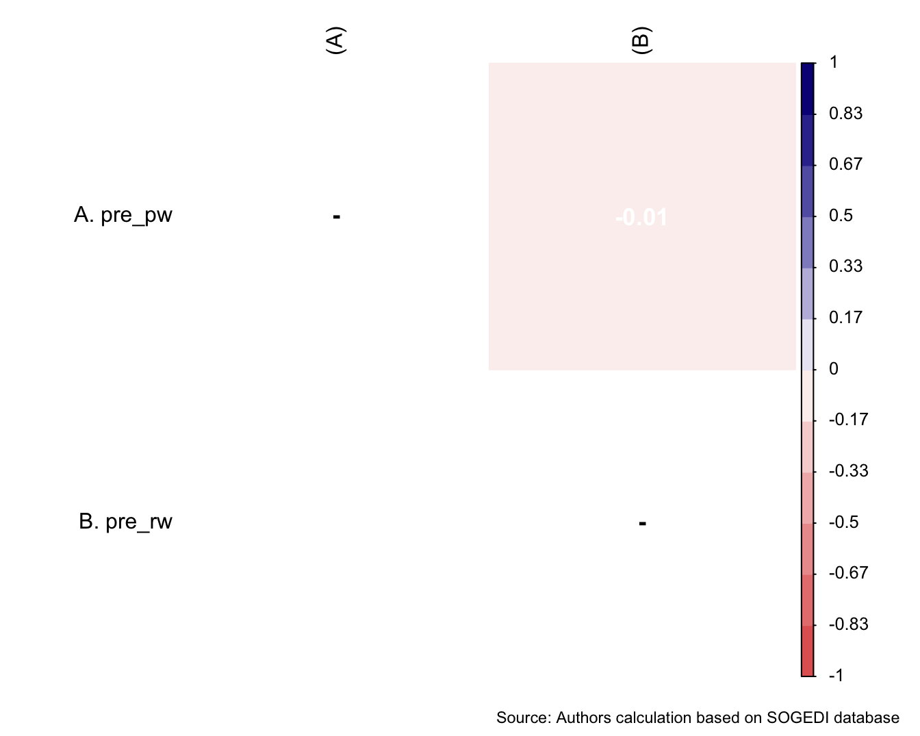
Reliability
mi_variable <- "pre"
result2 <- alphas(db_proc, c("pre_pw", "pre_rw"), mi_variable)Some items ( pre_rw ) were negatively correlated with the total scale and
probably should be reversed.
To do this, run the function again with the 'check.keys=TRUE' optionresult2$raw_alpha[1] -0.01070256result2$new_var_summary Min. 1st Qu. Median Mean 3rd Qu. Max.
1.000 4.000 4.000 4.327 5.000 7.000 5.8.4 Abuse of social assistance by poor mothers
The items to measure this process are inspired by scales on teenage mothers but we adapted to capture attitudes towards the group of poor mothers based on our experience with similar scales (Kim et al., 2013).
Descriptive analysis
describe_kable(db_proc, c("wel_abu_1","wel_abu_2"))| vars | n | mean | sd | median | trimmed | mad | min | max | range | skew | kurtosis | se | |
|---|---|---|---|---|---|---|---|---|---|---|---|---|---|
| wel_abu_1 | 1 | 4209 | 3.545 | 2.008 | 4 | 3.431 | 2.965 | 1 | 7 | 6 | 0.214 | -1.166 | 0.031 |
| wel_abu_2 | 2 | 4209 | 3.547 | 1.996 | 4 | 3.434 | 2.965 | 1 | 7 | 6 | 0.192 | -1.161 | 0.031 |
wrap_elements(
~corrplot::corrplot(
fit_correlations(db_proc, c("wel_abu_1","wel_abu_2")),
method = "color",
type = "upper",
col = colorRampPalette(c("#E16462", "white", "#0D0887"))(12),
tl.pos = "lt",
tl.col = "black",
addrect = 2,
rect.col = "black",
addCoef.col = "white",
cl.cex = 0.8,
cl.align.text = 'l',
number.cex = 1.1,
na.label = "-",
bg = "white"
)
) +
plot_annotation(
caption = paste0(
"Source: Authors calculation based on SOGEDI database"
)
)
Reliability
mi_variable <- "wel_abu"
result2 <- alphas(db_proc, c("wel_abu_1","wel_abu_2"), mi_variable)
result2$raw_alpha[1] 0.916503result2$new_var_summary Min. 1st Qu. Median Mean 3rd Qu. Max.
1.000 2.000 3.500 3.546 5.000 7.000 5.8.5 Paternalistic support for poor mothers
The items to measure this process are inspired by scales on teenage mothers but we adapted to capture attitudes towards the group of poor mothers based on our experience with similar scales (Kim et al., 2013).
Descriptive analysis
describe_kable(db_proc, c("wel_pa_1","wel_pa_2"))| vars | n | mean | sd | median | trimmed | mad | min | max | range | skew | kurtosis | se | |
|---|---|---|---|---|---|---|---|---|---|---|---|---|---|
| wel_pa_1 | 1 | 4209 | 6.036 | 1.542 | 7 | 6.368 | 0 | 1 | 7 | 6 | -1.718 | 2.265 | 0.024 |
| wel_pa_2 | 2 | 4209 | 6.008 | 1.478 | 7 | 6.303 | 0 | 1 | 7 | 6 | -1.617 | 2.081 | 0.023 |
wrap_elements(
~corrplot::corrplot(
fit_correlations(db_proc, c("wel_pa_1","wel_pa_2")),
method = "color",
type = "upper",
col = colorRampPalette(c("#E16462", "white", "#0D0887"))(12),
tl.pos = "lt",
tl.col = "black",
addrect = 2,
rect.col = "black",
addCoef.col = "white",
cl.cex = 0.8,
cl.align.text = 'l',
number.cex = 1.1,
na.label = "-",
bg = "white"
)
) +
plot_annotation(
caption = paste0(
"Source: Authors calculation based on SOGEDI database"
)
)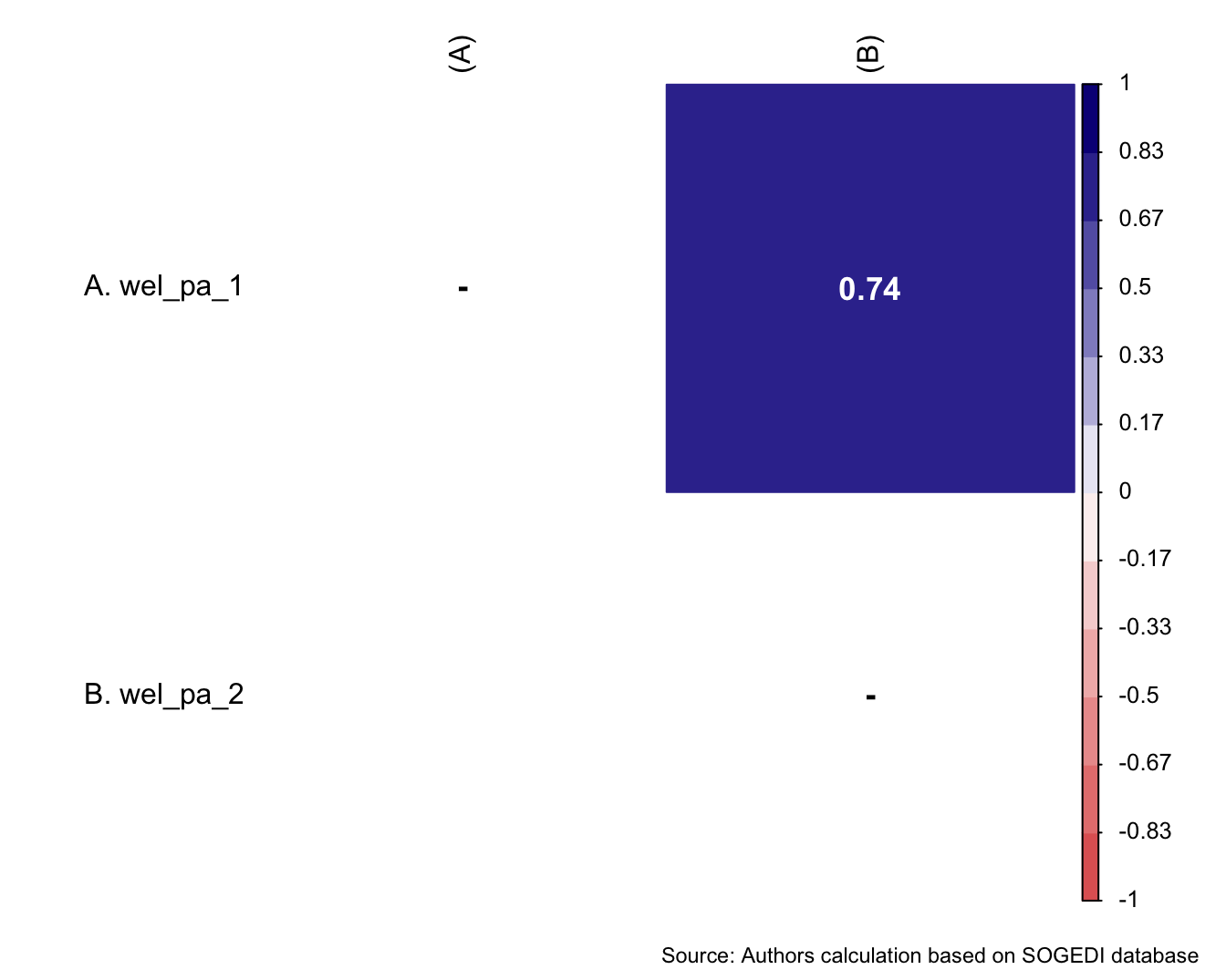
Reliability
mi_variable <- "wel_pa"
result2 <- alphas(db_proc, c("wel_pa_1","wel_pa_2"), mi_variable)
result2$raw_alpha[1] 0.8518911result2$new_var_summary Min. 1st Qu. Median Mean 3rd Qu. Max.
1.000 5.500 7.000 6.022 7.000 7.000 5.8.6 Hostile support for poor mothers
The items to measure this process are inspired by scales on teenage mothers but we adapted to capture attitudes towards the group of poor mothers based on our experience with similar scales (Kim et al., 2013).
Descriptive analysis
describe_kable(db_proc, c("wel_ho_1","wel_ho_2"))| vars | n | mean | sd | median | trimmed | mad | min | max | range | skew | kurtosis | se | |
|---|---|---|---|---|---|---|---|---|---|---|---|---|---|
| wel_ho_1 | 1 | 4209 | 3.730 | 2.312 | 4 | 3.663 | 4.448 | 1 | 7 | 6 | 0.139 | -1.473 | 0.036 |
| wel_ho_2 | 2 | 4209 | 4.434 | 2.249 | 5 | 4.542 | 2.965 | 1 | 7 | 6 | -0.310 | -1.335 | 0.035 |
wrap_elements(
~corrplot::corrplot(
fit_correlations(db_proc, c("wel_ho_1","wel_ho_2")),
method = "color",
type = "upper",
col = colorRampPalette(c("#E16462", "white", "#0D0887"))(12),
tl.pos = "lt",
tl.col = "black",
addrect = 2,
rect.col = "black",
addCoef.col = "white",
cl.cex = 0.8,
cl.align.text = 'l',
number.cex = 1.1,
na.label = "-",
bg = "white"
)
) +
plot_annotation(
caption = paste0(
"Source: Authors calculation based on SOGEDI database"
)
)
Reliability
mi_variable <- "wel_ho"
result2 <- alphas(db_proc, c("wel_ho_1","wel_ho_2"), mi_variable)
result2$raw_alpha[1] 0.825007result2$new_var_summary Min. 1st Qu. Median Mean 3rd Qu. Max.
1.000 2.000 4.000 4.082 6.000 7.000 5.9 Block 9. Policies / Actions
5.9.1 Support for income redistribution
Items adapted from García-Sánchez et al. (2022).
Descriptive analysis
describe_kable(db_proc, c("redi_1","redi_2"))| vars | n | mean | sd | median | trimmed | mad | min | max | range | skew | kurtosis | se | |
|---|---|---|---|---|---|---|---|---|---|---|---|---|---|
| redi_1 | 1 | 4209 | 4.795 | 1.984 | 5 | 4.993 | 2.965 | 1 | 7 | 6 | -0.530 | -0.834 | 0.031 |
| redi_2 | 2 | 4209 | 4.937 | 2.041 | 5 | 5.170 | 2.965 | 1 | 7 | 6 | -0.644 | -0.820 | 0.031 |
wrap_elements(
~corrplot::corrplot(
fit_correlations(db_proc, c("redi_1","redi_2")),
method = "color",
type = "upper",
col = colorRampPalette(c("#E16462", "white", "#0D0887"))(12),
tl.pos = "lt",
tl.col = "black",
addrect = 2,
rect.col = "black",
addCoef.col = "white",
cl.cex = 0.8,
cl.align.text = 'l',
number.cex = 1.1,
na.label = "-",
bg = "white"
)
) +
plot_annotation(
caption = paste0(
"Source: Authors calculation based on SOGEDI database"
)
)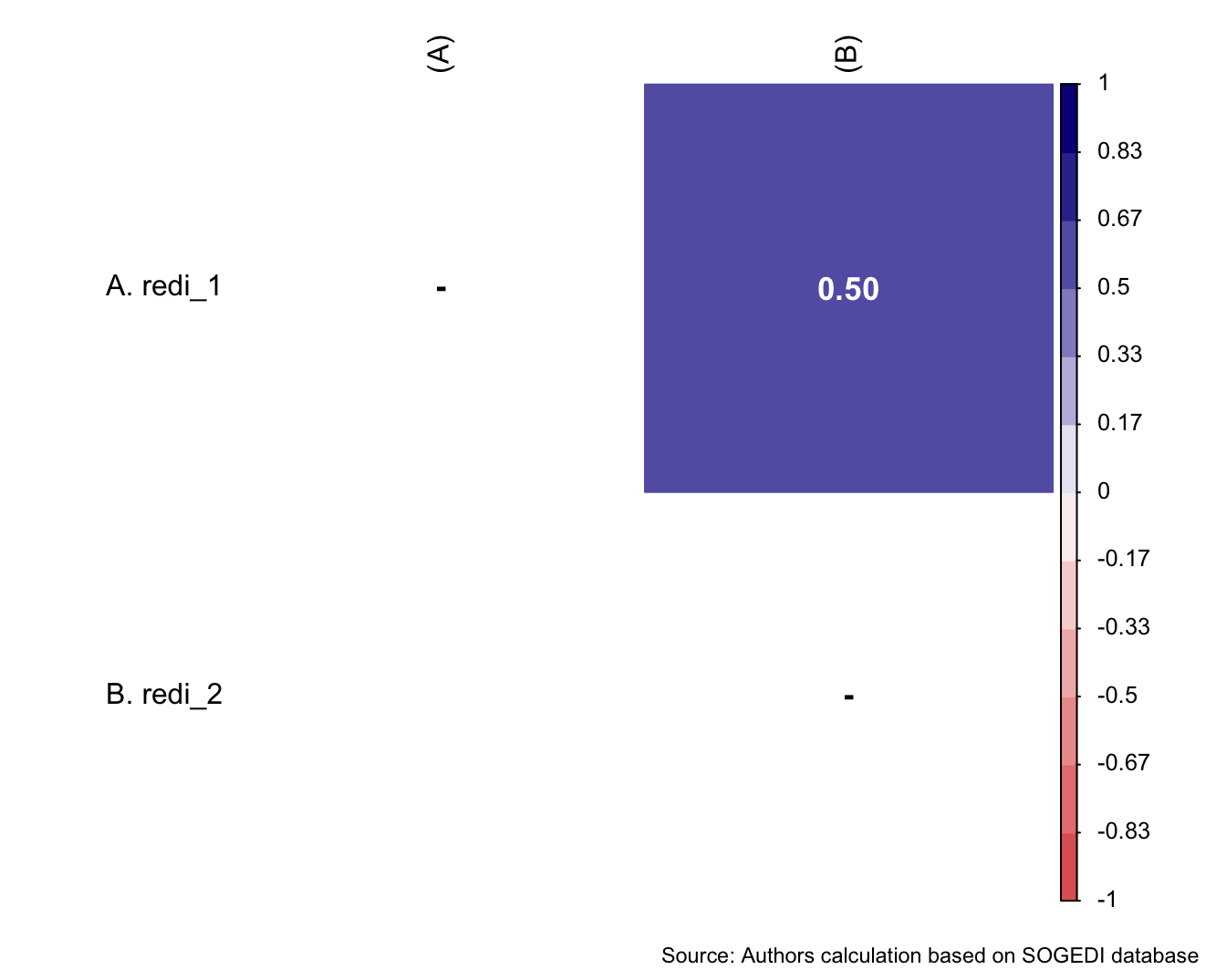
Reliability
5.9.2 Perception of effectiveness in the use of aids
Items previously used in Alcañiz-Colomer et al. (2023).
Descriptive analysis
describe_kable(db_proc, c("effec_pw_1", "effec_pw_2", "effec_pm_1", "effec_pm_2"))| vars | n | mean | sd | median | trimmed | mad | min | max | range | skew | kurtosis | se | |
|---|---|---|---|---|---|---|---|---|---|---|---|---|---|
| effec_pw_1 | 1 | 4209 | 3.852 | 1.796 | 4 | 3.824 | 1.483 | 1 | 7 | 6 | -0.010 | -0.865 | 0.028 |
| effec_pw_2 | 2 | 4209 | 4.239 | 1.514 | 4 | 4.243 | 1.483 | 1 | 7 | 6 | -0.026 | -0.358 | 0.023 |
| effec_pm_1 | 3 | 4209 | 4.334 | 1.735 | 4 | 4.397 | 1.483 | 1 | 7 | 6 | -0.264 | -0.718 | 0.027 |
| effec_pm_2 | 4 | 4209 | 3.920 | 1.473 | 4 | 3.895 | 1.483 | 1 | 7 | 6 | 0.121 | -0.234 | 0.023 |
wrap_elements(
~corrplot::corrplot(
fit_correlations(db_proc, c("effec_pw_1", "effec_pw_2", "effec_pm_1", "effec_pm_2")),
method = "color",
type = "upper",
col = colorRampPalette(c("#E16462", "white", "#0D0887"))(12),
tl.pos = "lt",
tl.col = "black",
addrect = 2,
rect.col = "black",
addCoef.col = "white",
cl.cex = 0.8,
cl.align.text = 'l',
number.cex = 1.1,
na.label = "-",
bg = "white"
)
) +
plot_annotation(
caption = paste0(
"Source: Authors calculation based on SOGEDI database"
)
)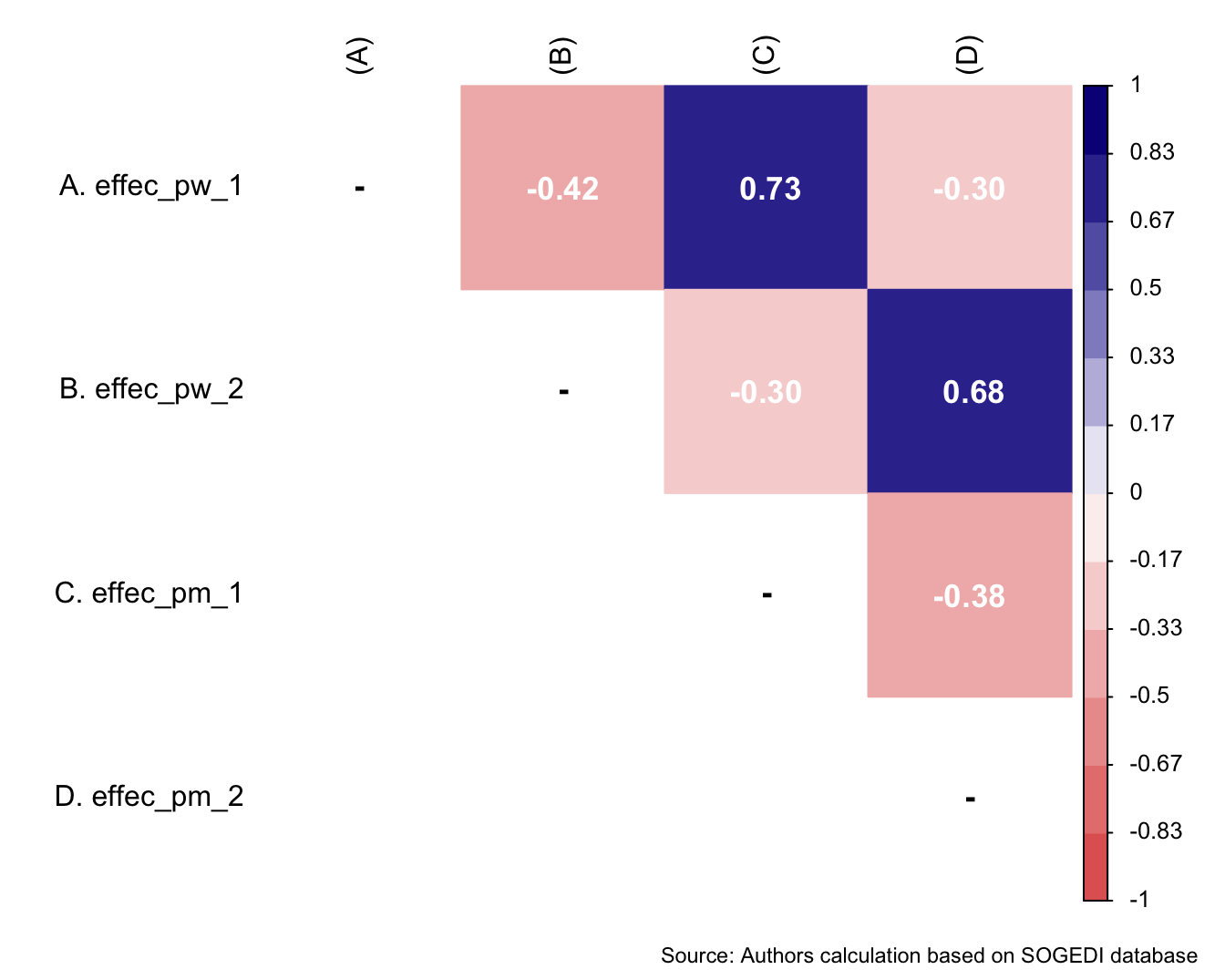
Reliability
mi_variable <- "effec_pw"
result2 <- psych::alpha(db_proc[,c("effec_pw_1", "effec_pw_2")], check.keys = T)
result2$total$raw_alpha[1] 0.5871212db_proc[[mi_variable]] <- rowMeans(db_proc[, c("effec_pw_1", "effec_pw_2")], na.rm = TRUE)
summary(db_proc$effec_pw) Min. 1st Qu. Median Mean 3rd Qu. Max.
1.000 3.500 4.000 4.046 4.500 7.000 mi_variable <- "effec_pm"
result2 <- psych::alpha(db_proc[,c("effec_pm_1", "effec_pm_2")], check.keys = T)
result2$total$raw_alpha[1] 0.541424db_proc[[mi_variable]] <- rowMeans(db_proc[, c("effec_pm_1", "effec_pm_2")], na.rm = TRUE)
summary(db_proc$effec_pw) Min. 1st Qu. Median Mean 3rd Qu. Max.
1.000 3.500 4.000 4.046 4.500 7.000 Confirmatory factor analysis
Mardia’s test for evaluate multivariate normality.
mardia(db_pw[,c("effec_pw_1", "effec_pw_2", "effec_pm_1", "effec_pm_2")],
na.rm = T, plot=T) Call: mardia(x = db_pw[, c(“effec_pw_1”, “effec_pw_2”, “effec_pm_1”, “effec_pm_2”)], na.rm = T, plot = T)
Mardia tests of multivariate skew and kurtosis Use describe(x) the to get univariate tests n.obs = 1052 num.vars = 4 b1p = 2.79 skew = 490.05 with probability <= 0.00000000000000000000000000000000000000000000000000000000000000000000000000000000000000000035 small sample skew = 492.01 with probability <= 0.00000000000000000000000000000000000000000000000000000000000000000000000000000000000000000014 b2p = 35.54 kurtosis = 27 with probability <= 0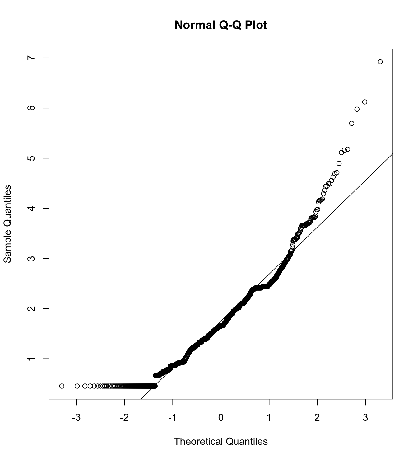
We first specify the factorial structure of the items, then fit models using a robust maximum likelihood estimator for the entire sample as well as for each country individually. The goodness of fit indicators are shown.
# model
model_cfa <- '
effectivness_pw =~ effec_pw_1 + effec_pw_2
effectivness_pm =~ effec_pm_1 + effec_pm_2
'
# estimation
m18_cfa <- cfa(model = model_cfa,
data = db_proc,
estimator = "MLR",
ordered = F,
std.lv = F)
m18_cfa_arg <- cfa(model = model_cfa,
data = subset(db_proc, country_residence_recoded == 1),
estimator = "MLR",
ordered = F,
std.lv = F)
m18_cfa_cl <- cfa(model = model_cfa,
data = subset(db_proc, country_residence_recoded == 3),
estimator = "MLR",
ordered = F,
std.lv = F)
m18_cfa_col <- cfa(model = model_cfa,
data = subset(db_proc, country_residence_recoded == 4),
estimator = "MLR",
ordered = F,
std.lv = F)
m18_cfa_es <- cfa(model = model_cfa,
data = subset(db_proc, country_residence_recoded == 9),
estimator = "MLR",
ordered = F,
std.lv = F)
m18_cfa_mex <- cfa(model = model_cfa,
data = subset(db_proc, country_residence_recoded == 13),
estimator = "MLR",
ordered = F,
std.lv = F) cfa_tab_fit(
models = list(m18_cfa, m18_cfa_cl, m18_cfa_mex),
country_names = c("Overall scores", "Chile", "México")
)$fit_table| \(N\) | Estimator | \(\chi^2\) (df) | CFI | TLI | RMSEA 90% CI [Lower-Upper] | SRMR | AIC | |
|---|---|---|---|---|---|---|---|---|
| Overall scores | 4209 | ML | 2478.502 (1) *** | 0.652 | -1.090 | 0.767 [0.742-0.793] | 0.154 | 59469.11 |
| Chile | 883 | ML | 479.246 (1) *** | 0.622 | -1.266 | 0.736 [0.681-0.792] | 0.161 | 12516.65 |
| México | 846 | ML | 381.487 (1) *** | 0.649 | -1.105 | 0.671 [0.615-0.728] | 0.158 | 12490.20 |
5.9.4 Progressive policies
Items comes from Jordan et al. (2021).
Descriptive analysis
describe_kable(db_proc, c("poli_progre_1", "poli_progre_2"))| vars | n | mean | sd | median | trimmed | mad | min | max | range | skew | kurtosis | se | |
|---|---|---|---|---|---|---|---|---|---|---|---|---|---|
| poli_progre_1 | 1 | 4209 | 5.562 | 1.655 | 6 | 5.827 | 1.483 | 1 | 7 | 6 | -1.051 | 0.352 | 0.026 |
| poli_progre_2 | 2 | 4209 | 5.793 | 1.472 | 6 | 6.024 | 1.483 | 1 | 7 | 6 | -1.180 | 0.842 | 0.023 |
wrap_elements(
~corrplot::corrplot(
fit_correlations(db_proc, c("poli_progre_1", "poli_progre_2")),
method = "color",
type = "upper",
col = colorRampPalette(c("#E16462", "white", "#0D0887"))(12),
tl.pos = "lt",
tl.col = "black",
addrect = 2,
rect.col = "black",
addCoef.col = "white",
cl.cex = 0.8,
cl.align.text = 'l',
number.cex = 1.1,
na.label = "-",
bg = "white"
)
) +
plot_annotation(
caption = paste0(
"Source: Authors calculation based on SOGEDI database"
)
)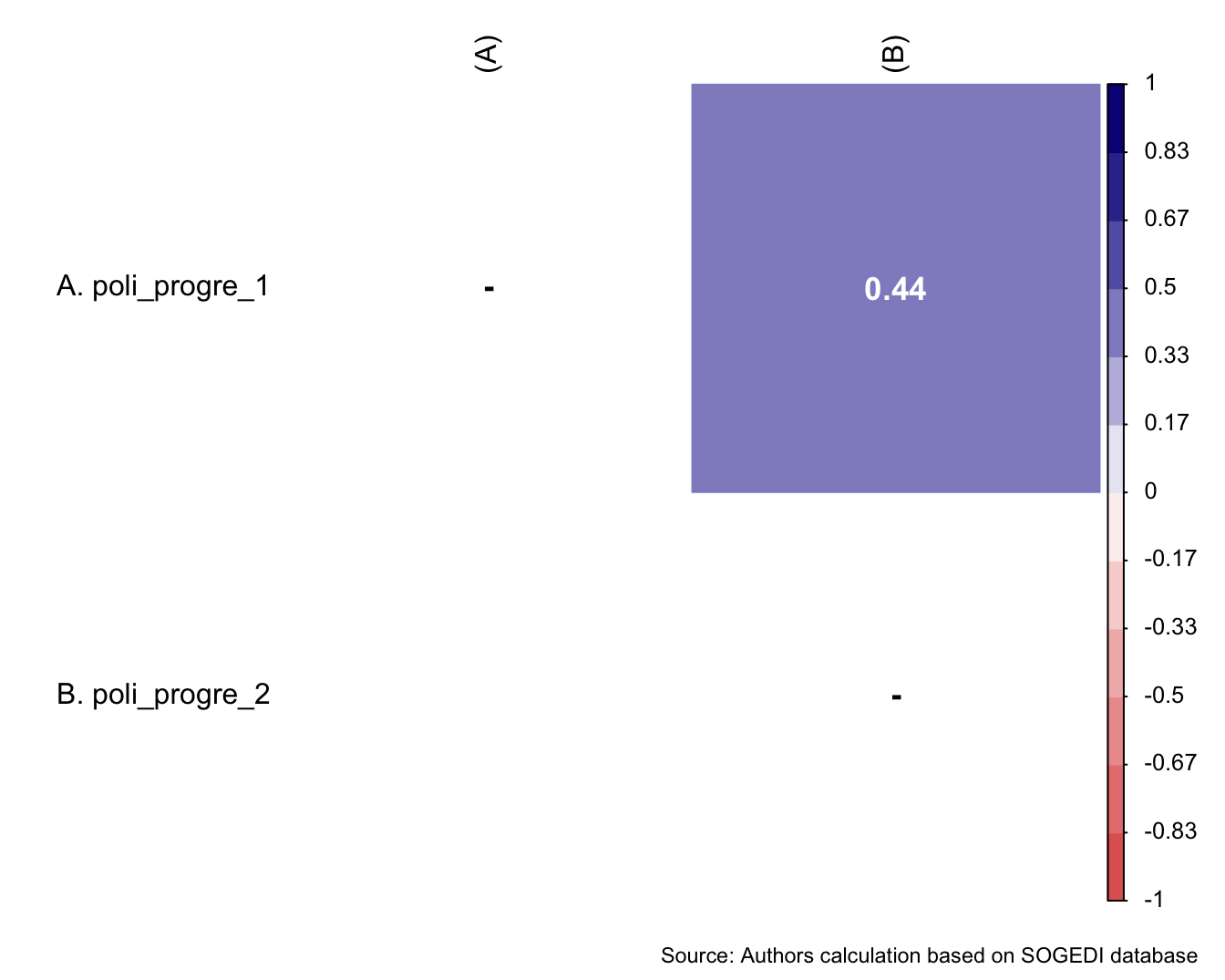
Reliability
mi_variable <- "poli_progre"
result2 <- alphas(db_proc, c("poli_progre_1", "poli_progre_2"), mi_variable)
result2$raw_alpha[1] 0.6076985result2$new_var_summary Min. 1st Qu. Median Mean 3rd Qu. Max.
1.000 5.000 6.000 5.678 7.000 7.000 5.9.5 Restrictive policies
Items comes from Jordan et al. (2021).
Descriptive analysis
describe_kable(db_proc, c("poli_restri_1", "poli_restri_2"))| vars | n | mean | sd | median | trimmed | mad | min | max | range | skew | kurtosis | se | |
|---|---|---|---|---|---|---|---|---|---|---|---|---|---|
| poli_restri_1 | 1 | 4209 | 4.906 | 2.102 | 5 | 5.132 | 2.965 | 1 | 7 | 6 | -0.648 | -0.896 | 0.032 |
| poli_restri_2 | 2 | 4209 | 4.850 | 1.923 | 5 | 5.048 | 2.965 | 1 | 7 | 6 | -0.551 | -0.771 | 0.030 |
wrap_elements(
~corrplot::corrplot(
fit_correlations(db_proc, c("poli_restri_1", "poli_restri_2")),
method = "color",
type = "upper",
col = colorRampPalette(c("#E16462", "white", "#0D0887"))(12),
tl.pos = "lt",
tl.col = "black",
addrect = 2,
rect.col = "black",
addCoef.col = "white",
cl.cex = 0.8,
cl.align.text = 'l',
number.cex = 1.1,
na.label = "-",
bg = "white"
)
) +
plot_annotation(
caption = paste0(
"Source: Authors calculation based on SOGEDI database"
)
)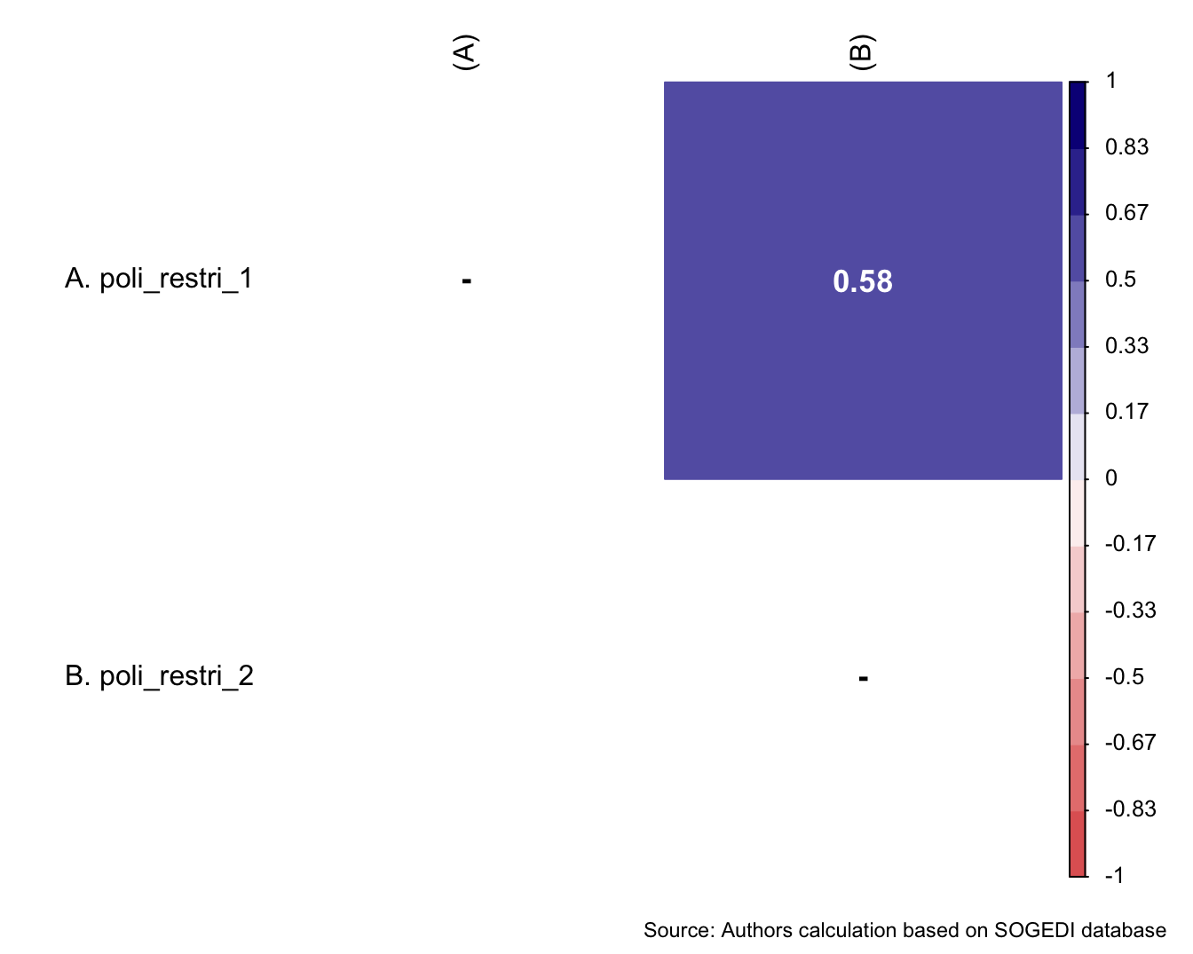
Reliability
mi_variable <- "poli_restri"
result2 <- alphas(db_proc, c("poli_restri_1", "poli_restri_2"), mi_variable)
result2$raw_alpha[1] 0.7332288result2$new_var_summary Min. 1st Qu. Median Mean 3rd Qu. Max.
1.000 4.000 5.000 4.878 6.500 7.000 5.10 Block 10. Violence
5.10.1 Sexual harassment situations
We used items from previous publications (Cheek et al., 2023) but slightly modified them to adapt to the context of the study.
Descriptive analysis
db_vio0 <- subset(db_proc, condi_viole == 0)
db_vio1 <- subset(db_proc, condi_viole == 1)
bind_rows(
psych::describe(db_vio0[,c("hara_pw_1", "hara_pw_2", "hara_pw_3")]) %>%
as_tibble() %>%
mutate(target = "Poor Women")
,
psych::describe(db_vio1[,c("hara_pw_1", "hara_pw_2", "hara_pw_3")]) %>%
as_tibble() %>%
mutate(target = "Rich Women")
) %>%
mutate(vars = paste0("hara_pw_", vars)) %>%
select(target, everything()) %>%
group_by(target) %>%
mutate(target = if_else(duplicated(target), NA, target)) %>%
kableExtra::kable(format = "markdown", digits = 3)| target | vars | n | mean | sd | median | trimmed | mad | min | max | range | skew | kurtosis | se |
|---|---|---|---|---|---|---|---|---|---|---|---|---|---|
| Poor Women | hara_pw_1 | 2100 | 5.669 | 1.626 | 6 | 5.940 | 1.483 | 1 | 7 | 6 | -1.109 | 0.346 | 0.035 |
| hara_pw_2 | 2100 | 6.420 | 1.146 | 7 | 6.713 | 0.000 | 1 | 7 | 6 | -2.242 | 4.774 | 0.025 | |
| hara_pw_3 | 2100 | 6.264 | 1.210 | 7 | 6.530 | 0.000 | 1 | 7 | 6 | -1.756 | 2.618 | 0.026 | |
| Rich Women | hara_pw_1 | 2109 | 5.685 | 1.663 | 6 | 5.978 | 1.483 | 1 | 7 | 6 | -1.190 | 0.548 | 0.036 |
| hara_pw_2 | 2109 | 6.365 | 1.190 | 7 | 6.658 | 0.000 | 1 | 7 | 6 | -2.148 | 4.458 | 0.026 | |
| hara_pw_3 | 2109 | 6.253 | 1.244 | 7 | 6.526 | 0.000 | 1 | 7 | 6 | -1.821 | 2.934 | 0.027 |
p1 <- wrap_elements(
~corrplot::corrplot(
fit_correlations(db_vio0, c("hara_pw_1", "hara_pw_2", "hara_pw_3")),
method = "color",
type = "upper",
col = colorRampPalette(c("#E16462", "white", "#0D0887"))(12),
tl.pos = "lt",
tl.col = "black",
addrect = 2,
rect.col = "black",
addCoef.col = "white",
cl.cex = 0.8,
cl.align.text = 'l',
number.cex = 1.1,
na.label = "-",
bg = "white"
)
) + labs(title = "I. Poor Women")
p2 <- wrap_elements(
~corrplot::corrplot(
fit_correlations(db_vio1, c("hara_pw_1", "hara_pw_2", "hara_pw_3")),
method = "color",
type = "upper",
col = colorRampPalette(c("#E16462", "white", "#0D0887"))(12),
tl.pos = "lt",
tl.col = "black",
addrect = 2,
rect.col = "black",
addCoef.col = "white",
cl.cex = 0.8,
cl.align.text = 'l',
number.cex = 1.1,
na.label = "-",
bg = "white"
)
) + labs(title = "II. Rich Women")
p1/p2 +
plot_annotation(
caption = paste0(
"Source: Authors calculation based on SOGEDI database"
)
)
Reliability
mi_variable <- "hara"
result2 <- alphas(db_proc, c("hara_pw_1", "hara_pw_2", "hara_pw_3"), mi_variable)
result2$raw_alpha[1] 0.8360801result2$new_var_summary Min. 1st Qu. Median Mean 3rd Qu. Max.
1.000 5.667 6.667 6.109 7.000 7.000 Confirmatory factor analysis
Mardia’s test for evaluate multivariate normality for each target.
mardia(db_vio0[,c("hara_pw_1", "hara_pw_2", "hara_pw_3")],
na.rm = T, plot=T) Call: mardia(x = db_vio0[, c(“hara_pw_1”, “hara_pw_2”, “hara_pw_3”)], na.rm = T, plot = T)
Mardia tests of multivariate skew and kurtosis Use describe(x) the to get univariate tests n.obs = 2100 num.vars = 3 b1p = 10.55 skew = 3693.64 with probability <= 0 small sample skew = 3701.56 with probability <= 0 b2p = 37.7 kurtosis = 94.97 with probability <= 0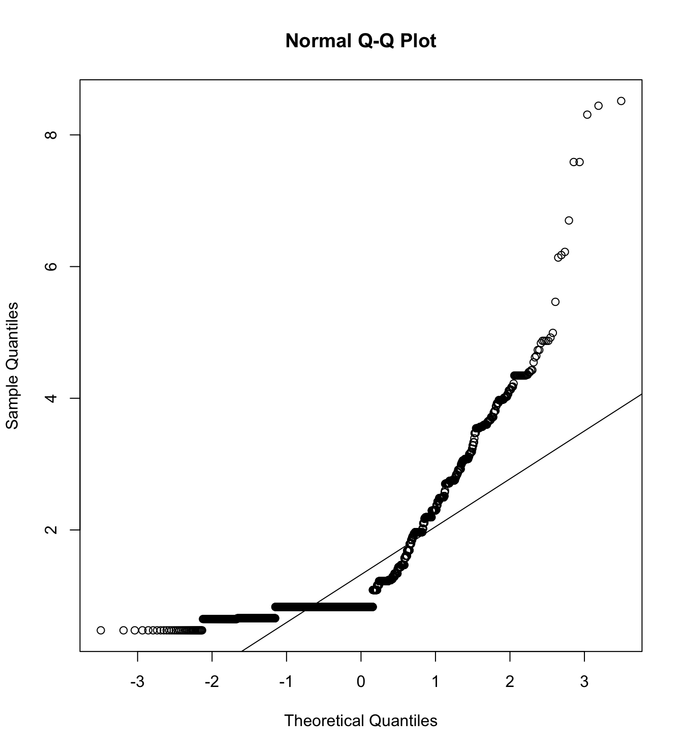
mardia(db_vio1[,c("hara_pw_1", "hara_pw_2", "hara_pw_3")],
na.rm = T, plot=T) Call: mardia(x = db_vio1[, c(“hara_pw_1”, “hara_pw_2”, “hara_pw_3”)], na.rm = T, plot = T)
Mardia tests of multivariate skew and kurtosis Use describe(x) the to get univariate tests n.obs = 2109 num.vars = 3 b1p = 10.3 skew = 3620.89 with probability <= 0 small sample skew = 3628.62 with probability <= 0 b2p = 38.49 kurtosis = 98.46 with probability <= 0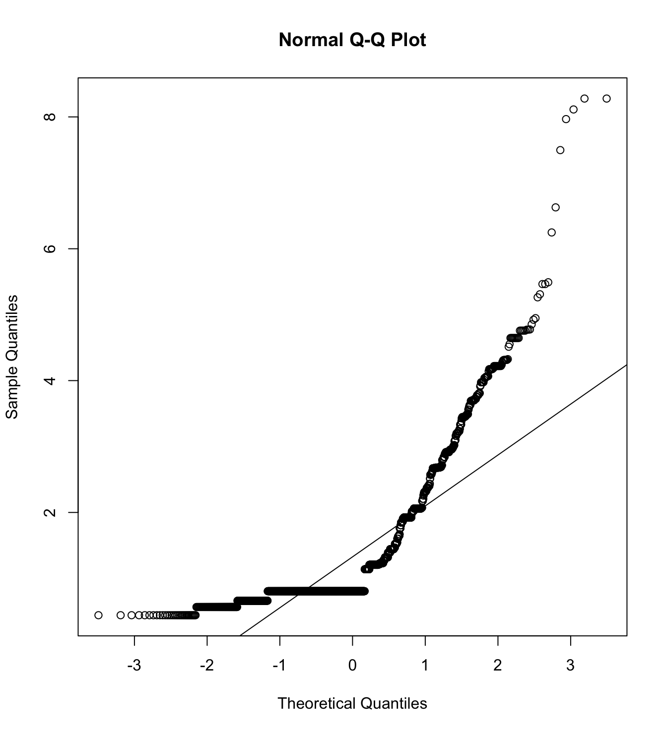
We first specify the factorial structure of the items, then fit models using a robust maximum likelihood estimator for the entire sample as well as for each country individually. The goodness of fit indicators are shown.
db_proc <- db_proc %>%
mutate(target = if_else(condi_viole == 0, "Poor.Women", "Rich.Women"))
# model
model_cfa <- '
harassment =~ hara_pw_1 + hara_pw_2 + hara_pw_3
'
# estimation
# overall
m19_cfa_rw <- cfa(model = model_cfa,
data = subset(db_proc, target == "Rich.Women"),
estimator = "MLR",
ordered = F,
std.lv = F)
m19_cfa_pw <- cfa(model = model_cfa,
data = subset(db_proc, target == "Poor.Women"),
estimator = "MLR",
ordered = F,
std.lv = F)
# per country
db_proc$group <- interaction(db_proc$natio_recoded, db_proc$target)
# argentina
m19_cfa_rw_arg <- cfa(model = model_cfa,
data = subset(db_proc, group == "1.Rich.Women"),
estimator = "MLR",
ordered = F,
std.lv = F)
m19_cfa_pw_arg <- cfa(model = model_cfa,
data = subset(db_proc, group == "1.Poor.Women"),
estimator = "MLR",
ordered = F,
std.lv = F)
# chile
m19_cfa_rw_cl <- cfa(model = model_cfa,
data = subset(db_proc, group == "3.Rich.Women"),
estimator = "MLR",
ordered = F,
std.lv = F)
m19_cfa_pw_cl <- cfa(model = model_cfa,
data = subset(db_proc, group == "3.Poor.Women"),
estimator = "MLR",
ordered = F,
std.lv = F)
# colombia
m19_cfa_rw_col <- cfa(model = model_cfa,
data = subset(db_proc, group == "4.Rich.Women"),
estimator = "MLR",
ordered = F,
std.lv = F)
m19_cfa_pw_col <- cfa(model = model_cfa,
data = subset(db_proc, group == "4.Poor.Women"),
estimator = "MLR",
ordered = F,
std.lv = F)
# españa
m19_cfa_rw_esp <- cfa(model = model_cfa,
data = subset(db_proc, group == "9.Rich.Women"),
estimator = "MLR",
ordered = F,
std.lv = F)
m19_cfa_pw_esp <- cfa(model = model_cfa,
data = subset(db_proc, group == "9.Poor.Women"),
estimator = "MLR",
ordered = F,
std.lv = F)
# mexico
m19_cfa_rw_mex <- cfa(model = model_cfa,
data = subset(db_proc, group == "13.Rich.Women"),
estimator = "MLR",
ordered = F,
std.lv = F)
m19_cfa_pw_mex <- cfa(model = model_cfa,
data = subset(db_proc, group == "13.Poor.Women"),
estimator = "MLR",
ordered = F,
std.lv = F) colnames_fit <- c("","Target","$N$","Estimator","$\\chi^2$ (df)","CFI","TLI","RMSEA 90% CI [Lower-Upper]", "SRMR", "AIC")
bind_rows(
cfa_tab_fit(
models = list(m19_cfa_rw, m19_cfa_rw_arg, m19_cfa_rw_cl, m19_cfa_rw_col, m19_cfa_rw_esp, m19_cfa_rw_mex),
country_names = c("Overall scores", "Argentina", "Chile", "Colombia", "Spain", "México")
)$sum_fit %>%
mutate(target = "Rich Women")
,
cfa_tab_fit(
models = list(m19_cfa_pw, m19_cfa_pw_arg, m19_cfa_pw_cl, m19_cfa_pw_col, m19_cfa_pw_esp, m19_cfa_pw_mex),
country_names = c("Overall scores", "Argentina", "Chile", "Colombia", "Spain", "México")
)$sum_fit %>%
mutate(target = "Poor Women")
) %>%
select(country, target, everything()) %>%
mutate(country = factor(country, levels = c("Overall scores", "Argentina", "Chile", "Colombia", "Spain", "México"))) %>%
group_by(country) %>%
arrange(country) %>%
mutate(country = if_else(duplicated(country), NA, country)) %>%
kableExtra::kable(
format = "markdown",
digits = 3,
booktabs = TRUE,
col.names = colnames_fit,
caption = NULL
) %>%
kableExtra::kable_styling(
full_width = TRUE,
font_size = 11,
latex_options = "HOLD_position",
bootstrap_options = c("striped", "bordered")
) %>%
kableExtra::collapse_rows(columns = 1)| Target | \(N\) | Estimator | \(\chi^2\) (df) | CFI | TLI | RMSEA 90% CI [Lower-Upper] | SRMR | AIC | |
|---|---|---|---|---|---|---|---|---|---|
| Overall scores | Rich Women | 2109 | ML | 0 (0) | 1 | 1 | 0 [0-0] | 0 | 18639.011 |
| Poor Women | 2100 | ML | 0 (0) | 1 | 1 | 0 [0-0] | 0 | 18278.000 | |
| Argentina | Rich Women | 427 | ML | 0 (0) | 1 | 1 | 0 [0-0] | 0 | 4000.984 |
| Poor Women | 430 | ML | 0 (0) | 1 | 1 | 0 [0-0] | 0 | 3816.214 | |
| Chile | Rich Women | 428 | ML | 0 (0) | 1 | 1 | 0 [0-0] | 0 | 3570.720 |
| Poor Women | 432 | ML | 0 (0) | 1 | 1 | 0 [0-0] | 0 | 3665.025 | |
| Colombia | Rich Women | 412 | ML | 0 (0) | 1 | 1 | 0 [0-0] | 0 | 3682.274 |
| Poor Women | 412 | ML | 0 (0) | 1 | 1 | 0 [0-0] | 0 | 3937.165 | |
| Spain | Rich Women | 417 | ML | 0 (0) | 1 | 1 | 0 [0-0] | 0 | 3646.568 |
| Poor Women | 414 | ML | 0 (0) | 1 | 1 | 0 [0-0] | 0 | 3448.210 | |
| México | Rich Women | 425 | ML | 0 (0) | 1 | 1 | 0 [0-0] | 0 | 3523.000 |
| Poor Women | 412 | ML | 0 (0) | 1 | 1 | 0 [0-0] | 0 | 3088.497 |
5.10.2 Domestic abuse situations
We used items from previous publications (Cheek et al., 2023) but slightly modified them to adapt to the context of the study. ##### Descriptive analysis
bind_rows(
psych::describe(db_vio0[,c("abu_pw_1", "abu_pw_2", "abu_pw_3")]) %>%
as_tibble() %>%
mutate(target = "Poor Women")
,
psych::describe(db_vio1[,c("abu_pw_1", "abu_pw_2", "abu_pw_3")]) %>%
as_tibble() %>%
mutate(target = "Rich Women")
) %>%
mutate(vars = paste0("hara_pw_", vars)) %>%
select(target, everything()) %>%
group_by(target) %>%
mutate(target = if_else(duplicated(target), NA, target)) %>%
kableExtra::kable(format = "markdown", digits = 3)| target | vars | n | mean | sd | median | trimmed | mad | min | max | range | skew | kurtosis | se |
|---|---|---|---|---|---|---|---|---|---|---|---|---|---|
| Poor Women | hara_pw_1 | 2100 | 6.449 | 1.126 | 7 | 6.737 | 0 | 1 | 7 | 6 | -2.328 | 5.260 | 0.025 |
| hara_pw_2 | 2100 | 6.560 | 1.041 | 7 | 6.848 | 0 | 1 | 7 | 6 | -2.722 | 7.461 | 0.023 | |
| hara_pw_3 | 2100 | 6.664 | 0.941 | 7 | 6.940 | 0 | 1 | 7 | 6 | -3.185 | 10.351 | 0.021 | |
| Rich Women | hara_pw_1 | 2109 | 6.501 | 1.038 | 7 | 6.764 | 0 | 1 | 7 | 6 | -2.518 | 6.713 | 0.023 |
| hara_pw_2 | 2109 | 6.636 | 0.929 | 7 | 6.896 | 0 | 1 | 7 | 6 | -3.096 | 10.384 | 0.020 | |
| hara_pw_3 | 2109 | 6.743 | 0.827 | 7 | 6.978 | 0 | 1 | 7 | 6 | -3.817 | 15.671 | 0.018 |
p1 <- wrap_elements(
~corrplot::corrplot(
fit_correlations(db_vio0, c("abu_pw_1", "abu_pw_2", "abu_pw_3")),
method = "color",
type = "upper",
col = colorRampPalette(c("#E16462", "white", "#0D0887"))(12),
tl.pos = "lt",
tl.col = "black",
addrect = 2,
rect.col = "black",
addCoef.col = "white",
cl.cex = 0.8,
cl.align.text = 'l',
number.cex = 1.1,
na.label = "-",
bg = "white"
)
) + labs(title = "I. Poor Women")
p2 <- wrap_elements(
~corrplot::corrplot(
fit_correlations(db_vio1, c("abu_pw_1", "abu_pw_2", "abu_pw_3")),
method = "color",
type = "upper",
col = colorRampPalette(c("#E16462", "white", "#0D0887"))(12),
tl.pos = "lt",
tl.col = "black",
addrect = 2,
rect.col = "black",
addCoef.col = "white",
cl.cex = 0.8,
cl.align.text = 'l',
number.cex = 1.1,
na.label = "-",
bg = "white"
)
) + labs(title = "II. Rich Women")
p1/p2 +
plot_annotation(
caption = paste0(
"Source: Authors calculation based on SOGEDI database"
)
)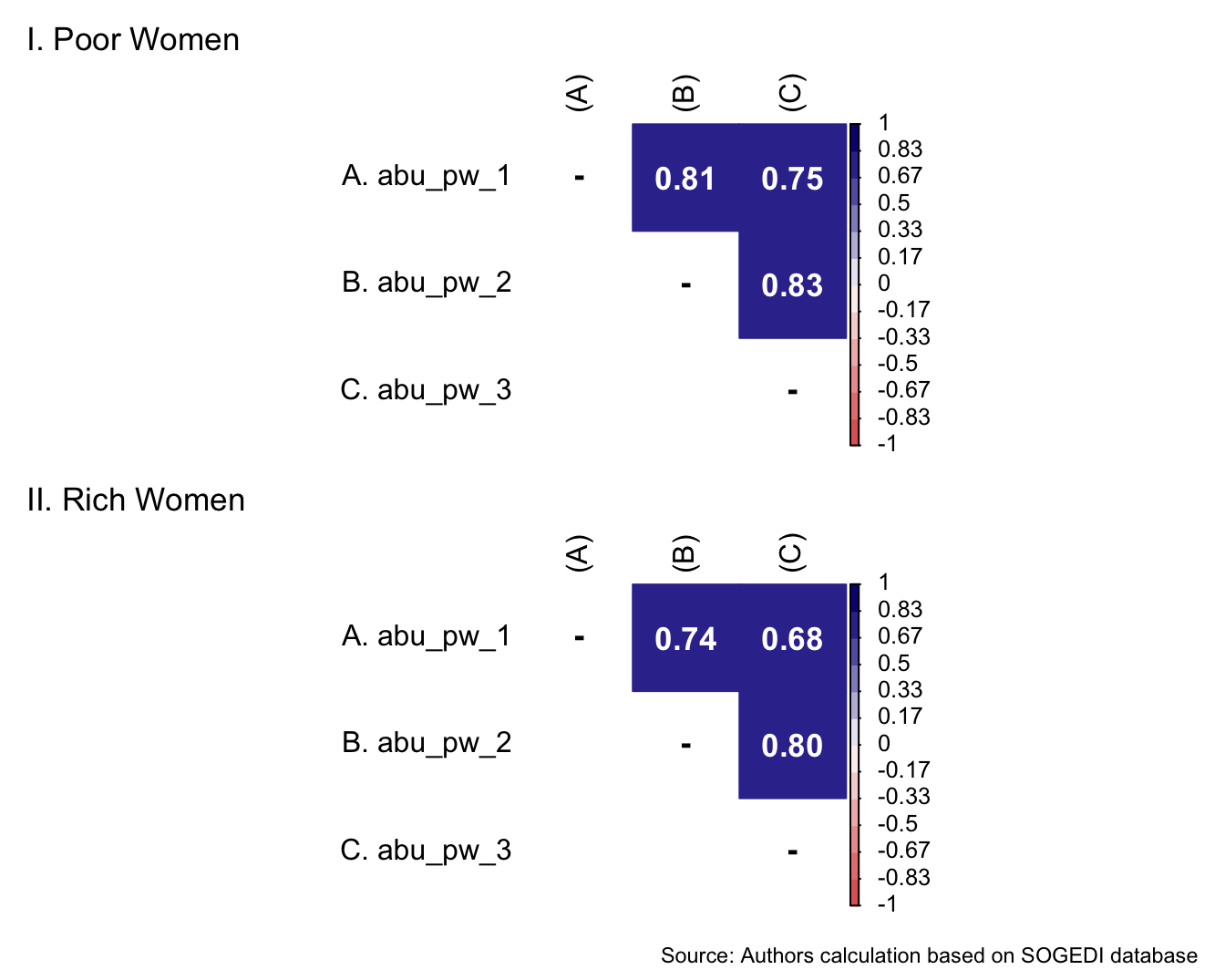
Reliability
mi_variable <- "abu"
result2 <- alphas(db_proc, c("abu_pw_1", "abu_pw_2", "abu_pw_3"), mi_variable)
result2$raw_alpha[1] 0.9074704result2$new_var_summary Min. 1st Qu. Median Mean 3rd Qu. Max.
1.000 6.667 7.000 6.592 7.000 7.000 Confirmatory factor analysis
Mardia’s test for evaluate multivariate normality for each target.
mardia(db_vio0[,c("abu_pw_1", "abu_pw_2", "abu_pw_3")],
na.rm = T, plot=T) Call: mardia(x = db_vio0[, c(“abu_pw_1”, “abu_pw_2”, “abu_pw_3”)], na.rm = T, plot = T)
Mardia tests of multivariate skew and kurtosis Use describe(x) the to get univariate tests n.obs = 2100 num.vars = 3 b1p = 26.1 skew = 9135.94 with probability <= 0 small sample skew = 9155.53 with probability <= 0 b2p = 80.82 kurtosis = 275.33 with probability <= 0
mardia(db_vio1[,c("abu_pw_1", "abu_pw_2", "abu_pw_3")],
na.rm = T, plot=T) Call: mardia(x = db_vio1[, c(“abu_pw_1”, “abu_pw_2”, “abu_pw_3”)], na.rm = T, plot = T)
Mardia tests of multivariate skew and kurtosis Use describe(x) the to get univariate tests n.obs = 2109 num.vars = 3 b1p = 34.23 skew = 12030.6 with probability <= 0 small sample skew = 12056.28 with probability <= 0 b2p = 90.31 kurtosis = 315.7 with probability <= 0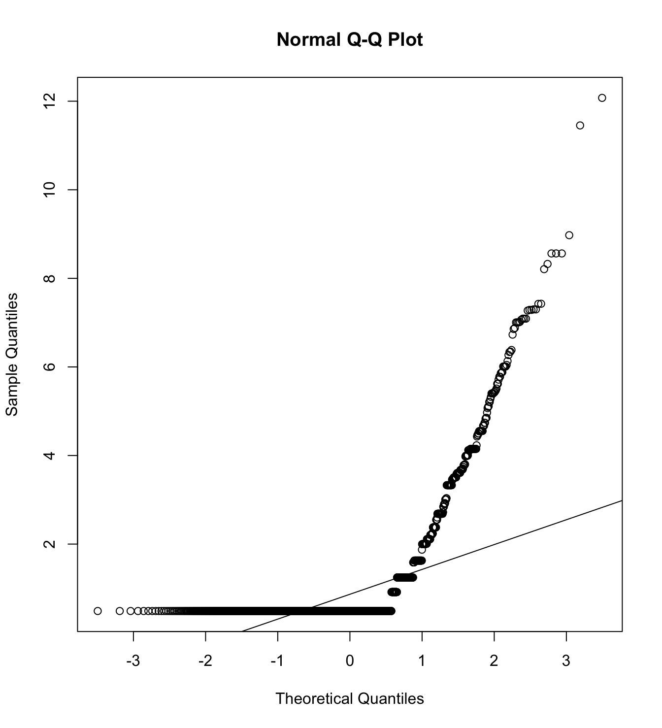
We first specify the factorial structure of the items, then fit models using a robust maximum likelihood estimator for the entire sample as well as for each country individually. The goodness of fit indicators are shown.
# model
model_cfa <- '
abuse =~ abu_pw_1 + abu_pw_2 + abu_pw_3
'
# estimation
# overall
m20_cfa_rw <- cfa(model = model_cfa,
data = subset(db_proc, target == "Rich.Women"),
estimator = "MLR",
ordered = F,
std.lv = F)
m20_cfa_pw <- cfa(model = model_cfa,
data = subset(db_proc, target == "Poor.Women"),
estimator = "MLR",
ordered = F,
std.lv = F)
# argentina
m20_cfa_rw_arg <- cfa(model = model_cfa,
data = subset(db_proc, group == "1.Rich.Women"),
estimator = "MLR",
ordered = F,
std.lv = F)
m20_cfa_pw_arg <- cfa(model = model_cfa,
data = subset(db_proc, group == "1.Poor.Women"),
estimator = "MLR",
ordered = F,
std.lv = F)
# chile
m20_cfa_rw_cl <- cfa(model = model_cfa,
data = subset(db_proc, group == "3.Rich.Women"),
estimator = "MLR",
ordered = F,
std.lv = F)
m20_cfa_pw_cl <- cfa(model = model_cfa,
data = subset(db_proc, group == "3.Poor.Women"),
estimator = "MLR",
ordered = F,
std.lv = F)
# colombia
m20_cfa_rw_col <- cfa(model = model_cfa,
data = subset(db_proc, group == "4.Rich.Women"),
estimator = "MLR",
ordered = F,
std.lv = F)
m20_cfa_pw_col <- cfa(model = model_cfa,
data = subset(db_proc, group == "4.Poor.Women"),
estimator = "MLR",
ordered = F,
std.lv = F)
# españa
m20_cfa_rw_esp <- cfa(model = model_cfa,
data = subset(db_proc, group == "9.Rich.Women"),
estimator = "MLR",
ordered = F,
std.lv = F)
m20_cfa_pw_esp <- cfa(model = model_cfa,
data = subset(db_proc, group == "9.Poor.Women"),
estimator = "MLR",
ordered = F,
std.lv = F)
# mexico
m20_cfa_rw_mex <- cfa(model = model_cfa,
data = subset(db_proc, group == "13.Rich.Women"),
estimator = "MLR",
ordered = F,
std.lv = F)
m20_cfa_pw_mex <- cfa(model = model_cfa,
data = subset(db_proc, group == "13.Poor.Women"),
estimator = "MLR",
ordered = F,
std.lv = F) colnames_fit <- c("","Target","$N$","Estimator","$\\chi^2$ (df)","CFI","TLI","RMSEA 90% CI [Lower-Upper]", "SRMR", "AIC")
bind_rows(
cfa_tab_fit(
models = list(m20_cfa_rw, m20_cfa_rw_arg, m20_cfa_rw_cl, m20_cfa_rw_col, m20_cfa_rw_esp, m20_cfa_rw_mex),
country_names = c("Overall scores", "Argentina", "Chile", "Colombia", "Spain", "México")
)$sum_fit %>%
mutate(target = "Rich Women")
,
cfa_tab_fit(
models = list(m20_cfa_pw, m20_cfa_pw_arg, m20_cfa_pw_cl, m20_cfa_pw_col, m20_cfa_pw_esp, m20_cfa_pw_mex),
country_names = c("Overall scores", "Argentina", "Chile", "Colombia", "Spain", "México")
)$sum_fit %>%
mutate(target = "Poor Women")
) %>%
select(country, target, everything()) %>%
mutate(country = factor(country, levels = c("Overall scores", "Argentina", "Chile", "Colombia", "Spain", "México"))) %>%
group_by(country) %>%
arrange(country) %>%
mutate(country = if_else(duplicated(country), NA, country)) %>%
kableExtra::kable(
format = "markdown",
digits = 3,
booktabs = TRUE,
col.names = colnames_fit,
caption = NULL
) %>%
kableExtra::kable_styling(
full_width = TRUE,
font_size = 11,
latex_options = "HOLD_position",
bootstrap_options = c("striped", "bordered")
) %>%
kableExtra::collapse_rows(columns = 1)| Target | \(N\) | Estimator | \(\chi^2\) (df) | CFI | TLI | RMSEA 90% CI [Lower-Upper] | SRMR | AIC | |
|---|---|---|---|---|---|---|---|---|---|
| Overall scores | Rich Women | 2109 | ML | 0 (0) | 1 | 1 | 0 [0-0] | 0 | 13016.345 |
| Poor Women | 2100 | ML | 0 (0) | 1 | 1 | 0 [0-0] | 0 | 13440.990 | |
| Argentina | Rich Women | 427 | ML | 0 (0) | 1 | 1 | 0 [0-0] | 0 | 2467.874 |
| Poor Women | 430 | ML | 0 (0) | 1 | 1 | 0 [0-0] | 0 | 2687.205 | |
| Chile | Rich Women | 428 | ML | 0 (0) | 1 | 1 | 0 [0-0] | 0 | 2638.312 |
| Poor Women | 432 | ML | 0 (0) | 1 | 1 | 0 [0-0] | 0 | 2840.373 | |
| Colombia | Rich Women | 412 | ML | 0 (0) | 1 | 1 | 0 [0-0] | 0 | 2790.489 |
| Poor Women | 412 | ML | 0 (0) | 1 | 1 | 0 [0-0] | 0 | 2997.369 | |
| Spain | Rich Women | 417 | ML | 0 (0) | 1 | 1 | 0 [0-0] | 0 | 1998.865 |
| Poor Women | 414 | ML | 0 (0) | 1 | 1 | 0 [0-0] | 0 | 1841.201 | |
| México | Rich Women | 425 | ML | 0 (0) | 1 | 1 | 0 [0-0] | 0 | 2783.450 |
| Poor Women | 412 | ML | 0 (0) | 1 | 1 | 0 [0-0] | 0 | 2652.700 |
5.10.3 Type of violence
We have created these items with the purpose of determining if there are differences in the type of violence perceived associated with each social class. ##### Descriptive analysis
describe_kable(db_proc, c("viole_pw_1", "viole_pw_2", "viole_pw_3", "viole_pw_4", "viole_pw_5", "viole_pw_6"))| vars | n | mean | sd | median | trimmed | mad | min | max | range | skew | kurtosis | se | |
|---|---|---|---|---|---|---|---|---|---|---|---|---|---|
| viole_pw_1 | 1 | 4209 | 5.499 | 1.530 | 6 | 5.705 | 1.483 | 1 | 7 | 6 | -0.830 | -0.017 | 0.024 |
| viole_pw_2 | 2 | 4209 | 5.707 | 1.437 | 6 | 5.910 | 1.483 | 1 | 7 | 6 | -1.024 | 0.484 | 0.022 |
| viole_pw_3 | 3 | 4209 | 5.707 | 1.462 | 6 | 5.926 | 1.483 | 1 | 7 | 6 | -1.082 | 0.583 | 0.023 |
| viole_pw_4 | 4 | 4209 | 5.425 | 1.594 | 6 | 5.632 | 1.483 | 1 | 7 | 6 | -0.797 | -0.184 | 0.025 |
| viole_pw_5 | 5 | 4209 | 5.363 | 1.741 | 6 | 5.616 | 1.483 | 1 | 7 | 6 | -0.892 | -0.154 | 0.027 |
| viole_pw_6 | 6 | 4209 | 5.445 | 1.606 | 6 | 5.668 | 1.483 | 1 | 7 | 6 | -0.882 | 0.027 | 0.025 |
5.10.4 Barriers to leaving an abusive relationship
We have created these items with the purpose of determining if there are differences in the type of barriers associated with leaving an abusive relationship each social class. ##### Descriptive analysis
describe_kable(db_proc, c("barri_pw_1", "barri_pw_2", "barri_pw_3", "barri_pw_4", "barri_pw_5"))| vars | n | mean | sd | median | trimmed | mad | min | max | range | skew | kurtosis | se | |
|---|---|---|---|---|---|---|---|---|---|---|---|---|---|
| barri_pw_1 | 1 | 4209 | 5.552 | 1.534 | 6 | 5.776 | 1.483 | 1 | 7 | 6 | -0.944 | 0.202 | 0.024 |
| barri_pw_2 | 2 | 4209 | 5.402 | 1.767 | 6 | 5.680 | 1.483 | 1 | 7 | 6 | -0.968 | -0.073 | 0.027 |
| barri_pw_3 | 3 | 4209 | 5.249 | 1.624 | 5 | 5.428 | 1.483 | 1 | 7 | 6 | -0.683 | -0.304 | 0.025 |
| barri_pw_4 | 4 | 4209 | 5.012 | 1.819 | 5 | 5.207 | 1.483 | 1 | 7 | 6 | -0.612 | -0.645 | 0.028 |
| barri_pw_5 | 5 | 4209 | 5.530 | 1.482 | 6 | 5.723 | 1.483 | 1 | 7 | 6 | -0.895 | 0.255 | 0.023 |
5.10.5 Perpetration of violence
Exploratory items were developed by the project team.
Descriptive analysis
describe_kable(db_proc, c("perpe_1", "perpe_2", "perpe_3", "perpe_4", "perpe_5"))| vars | n | mean | sd | median | trimmed | mad | min | max | range | skew | kurtosis | se | |
|---|---|---|---|---|---|---|---|---|---|---|---|---|---|
| perpe_1 | 1 | 4209 | 1.158 | 0.572 | 1 | 1.000 | 0 | 1 | 5 | 4 | 4.171 | 18.588 | 0.009 |
| perpe_2 | 2 | 4209 | 1.383 | 0.762 | 1 | 1.194 | 0 | 1 | 5 | 4 | 2.282 | 5.410 | 0.012 |
| perpe_3 | 3 | 4209 | 1.135 | 0.546 | 1 | 1.000 | 0 | 1 | 5 | 4 | 4.670 | 23.259 | 0.008 |
| perpe_4 | 4 | 4209 | 1.465 | 0.800 | 1 | 1.288 | 0 | 1 | 5 | 4 | 1.866 | 3.372 | 0.012 |
| perpe_5 | 5 | 4209 | 1.119 | 0.519 | 1 | 1.000 | 0 | 1 | 5 | 4 | 5.098 | 27.932 | 0.008 |
Reliability
mi_variable <- "perpe"
result2 <- alphas(db_proc, c("perpe_1", "perpe_2", "perpe_3", "perpe_4", "perpe_5"), mi_variable)
result2$raw_alpha[1] 0.8855049result2$new_var_summary Min. 1st Qu. Median Mean 3rd Qu. Max.
1.000 1.000 1.000 1.252 1.200 5.000 Confirmatory factor analysis
Mardia’s test for evaluate multivariate normality.
mardia(db_proc[,c("perpe_1", "perpe_2", "perpe_3", "perpe_4", "perpe_5")],
na.rm = T, plot=T) Call: mardia(x = db_proc[, c(“perpe_1”, “perpe_2”, “perpe_3”, “perpe_4”, “perpe_5”)], na.rm = T, plot = T)
Mardia tests of multivariate skew and kurtosis Use describe(x) the to get univariate tests n.obs = 4209 num.vars = 5 b1p = 61.96 skew = 43465.5 with probability <= 0 small sample skew = 43506.82 with probability <= 0 b2p = 176.96 kurtosis = 550.38 with probability <= 0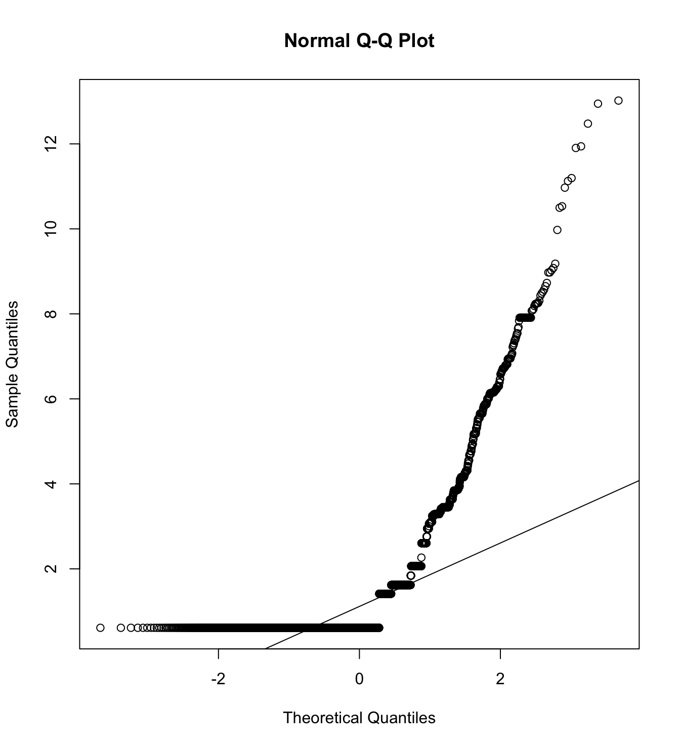
We first specify the factorial structure of the items, then fit models using a robust maximum likelihood estimator for the entire sample as well as for each country individually. The goodness of fit indicators are shown.
# model
model_cfa <- ' perpe_viole =~ perpe_1 + perpe_2 + perpe_3 + perpe_4 + perpe_5 '
# estimation
m21_cfa <- cfa(model = model_cfa,
data = db_proc,
estimator = "MLR",
ordered = F,
std.lv = F)
m21_cfa_arg <- cfa(model = model_cfa,
data = subset(db_proc, country_residence_recoded == 1),
estimator = "MLR",
ordered = F,
std.lv = F)
m21_cfa_cl <- cfa(model = model_cfa,
data = subset(db_proc, country_residence_recoded == 3),
estimator = "MLR",
ordered = F,
std.lv = F)
m21_cfa_col <- cfa(model = model_cfa,
data = subset(db_proc, country_residence_recoded == 4),
estimator = "MLR",
ordered = F,
std.lv = F)
m21_cfa_es <- cfa(model = model_cfa,
data = subset(db_proc, country_residence_recoded == 9),
estimator = "MLR",
ordered = F,
std.lv = F)
m21_cfa_mex <- cfa(model = model_cfa,
data = subset(db_proc, country_residence_recoded == 13),
estimator = "MLR",
ordered = F,
std.lv = F) cfa_tab_fit(
models = list(m21_cfa, m21_cfa_arg, m21_cfa_cl, m21_cfa_col, m21_cfa_es, m21_cfa_mex),
country_names = c("Overall scores", "Argentina", "Chile", "Colombia", "Spain", "México")
)$fit_table| \(N\) | Estimator | \(\chi^2\) (df) | CFI | TLI | RMSEA 90% CI [Lower-Upper] | SRMR | AIC | |
|---|---|---|---|---|---|---|---|---|
| Overall scores | 4209 | ML | 1268.801 (5) *** | 0.908 | 0.816 | 0.245 [0.234-0.256] | 0.065 | 27755.146 |
| Argentina | 807 | ML | 355.444 (5) *** | 0.854 | 0.708 | 0.295 [0.269-0.321] | 0.094 | 4731.560 |
| Chile | 883 | ML | 263.913 (5) *** | 0.901 | 0.802 | 0.242 [0.218-0.267] | 0.067 | 5557.754 |
| Colombia | 833 | ML | 242.026 (5) *** | 0.920 | 0.840 | 0.239 [0.213-0.265] | 0.056 | 5916.789 |
| Spain | 835 | ML | 302.777 (5) *** | 0.899 | 0.797 | 0.267 [0.242-0.293] | 0.082 | 3335.810 |
| México | 846 | ML | 227.252 (5) *** | 0.925 | 0.849 | 0.229 [0.204-0.255] | 0.049 | 6964.814 |
5.9.3 Social aids that promote autonomy vs. dependence
Single item based on Sainz et al. (2020) about governmental control of social welfare spending. This is supposed to capture dependence assistance towards poor men/women. We selected the item from Alcañiz-Colomer et al. (2023) that worked best and most clearly represents dependence vs. autonomy.
Descriptive analysis